Distributed Fusion Receding Horizon Filtering in Linear Stochastic Systems

(1)

Volume 2009, Article ID 929535,8pages doi:10.1155/2009/929535

Research Article

Distributed Fusion Receding Horizon Filtering in

Linear Stochastic Systems

Il Young Song,

1

_{Du Yong Kim,}

1

_{Yong Hoon Kim,}

1

_{Suk Jae Lee,}

2

_{and Vladimir Shin}

1

1_{School of Information and Mechatronics, Gwangju Institute of Science and Technology, 1 Oryong-Dong, Buk-Gu,} Gwangju 500-712, South Korea

2_{Agency for Defense Development (ADD), Jochiwongil 462, Yuseong, Daejeon 305-152, South Korea}

Correspondence should be addressed to Vladimir Shin,[email protected]

Received 5 May 2009; Accepted 21 September 2009

Recommended by Fredrik Gustafsson

This paper presents a distributed receding horizon filtering algorithm for multisensor continuous-time linear stochastic systems. Distributed fusion with a weighted sum structure is applied to local receding horizon Kalman filters having different horizon lengths. The fusion estimate of the state of a dynamic system represents the optimal linear fusion by weighting matrices under the minimum mean square error criterion. The key contribution of this paper lies in the derivation of the differential equations for determining the error cross-covariances between the local receding horizon Kalman filters. The subsequent application of the proposed distributed filter to a linear dynamic system within a multisensor environment demonstrates its effectiveness.

Copyright © 2009 Il Young Song et al. This is an open access article distributed under the Creative Commons Attribution License, which permits unrestricted use, distribution, and reproduction in any medium, provided the original work is properly cited.

1. Introduction

The concept of multisensor data fusion is the combination of data generated by a number of sensors in order to obtain more valuable data and perform inferences that may not be possible from a single sensor alone. This process has attracted growing interest for its potential applications in areas such as robotics, aerospace, and environmental monitoring, among others [1,2].

In general, there are two fusion estimation methods commonly used to process the measured sensor data [3,4]. If a central processor directly receives the measurement data of all local sensors and processes them in real time, the correlative result is known as the centralized estimation. However, this approach has some serious disadvantages, including bad reliability and survivability, as well as heavy communication and computational burdens.

The second method is called distributed estimation fusion, in which every local sensor is attached to a local processor. In this method, the processor optimally estimates a parameter or state of a system based on its own local measurements and transmits its local estimate to the fusion center where the received information is suitably associated to yield the global inference. The advantage of this approach

is that the parallel structures would cause enlarge the input data rates and make easy fault detection and isolation [1–5]. Recently, various distributed and parallel versions of standard Kalman filters have been reported for linear dynamic systems within a multisensor environment [6–10].

(2)

typically more robust against dynamic model uncertainties and numerical errors than standard local Kalman filters, which utilize all measurements [14–17].

Distributed receding horizon fusion filtering for multiple sensors with equal horizon time intervals (horizon lengths) has also been proposed in [16]. In this case, all LRHKFs with the same horizon time interval, which are fused, utilize finite measurements over the most recent time interval [12–16].

In this paper, we consider the generalization of [16] for arbitrary, nonequal horizon lengths. Design of distributed filters for sensor measurements with nonequal horizon lengths is generally more complicated than for equal lengths due to a lack of common time intervals that contain all sensor data, making it impossible to design a centralized filtering algorithm. We propose using a distributed receding horizon filter for a set of local sensors with nonequal horizon lengths. Also, we derive the key diﬀerential equations for error cross-covariances between LRHKFs using diﬀerent horizon lengths.

The remainder of this paper is organized as follows. The problem setting is described inSection 2. In Section 3, we present the main results pertaining to the distributed reced-ing horizon filterreced-ing for a multisensor environment. Here, the key equations for cross-covariances between the local receding horizon filtering errors are derived. In Section 4, two examples for continuous-time dynamic systems within a multisensor environment illustrate the main results, and concluding remarks are then given inSection 5.

2. Problem Setting

Consider the linear continuous-time dynamic system withN

sensors:

˙

xt=Ftxt+Gtvt, x0=xt0, t≥t0, (1)

y(ti)=H( i)

t xt+w(ti), i=1,. . .,N, (2)

wherext ∈Rnis the state,yt(i) ∈Rmi is the measurement,

the system noise vt ∈ Rr and the measurement noises

wt(i) ∈ Rmi,i = 1,. . .,N are uncorrelated white Gaussian

noises with zero mean and intensity matrices Qt and

R(ti), respectively, and Ft, Gt, and Ht(i) are matrices with

compatible dimensions. Also, the superscript (i) denotes the

ith sensor, andNis the total number of sensors.

The initial state x0 ∼ N(m0;P0), m0 = E(x0), P0 =

cov{x0,x0}is assumed to be Gaussian and uncorrelated with vtandw(ti),i=1,. . .,N.

Our purpose, then, is to find the distributed fusion estimate of the statext based on the overall horizon sensor

measurementsYt with diﬀerent horizon time intervals Δi,

i=1,. . .,N, such that

Yt=

Yt(1),. . .,Yt(N)

,

Yt(i)=

y(i)

s :t−Δi≤s≤t

, i=1,. . .,N .

(3)

3. Distributed Fusion Receding Horizon Filter

Now, we will show that the fusion formula (FF) [10,17] is able to serve as the basis for designing a distributed fusion filter. A newdistributed fusion receding horizon filter with nonequal horizon lengths (NE-DFRHF) includes two stages. In the first stage, LRHKFs (estimates)xt(1),. . .,x(

N)

t are

computed and then linearly fused at the second stage based on the FF.

First step (Calculation of LRHKFs). According to (1) and (2), we haveNlocal dynamic subsystems with the state vectorxt

and local (individual) sensor measurementyt(i):

˙

xt=Ftxt+Gtvt, x0=xt0,

yt(i)=Ht(i)xt+wt(i),

(4)

where the numberiof a local subsystem is fixed.

Next, let us denote the local receding horizon estimate of the statext based on the individual sensor measurements

Yt(i) = {ys(i) : t−Δi ≤ s ≤ t}by xt(i). To determine x(ti)

we can apply the optimal receding horizon Kalman filter to subsystem (4) [12–15] to obtain the following diﬀerential equations:

˙

xs(i)=Fsxs(i)+Ks(i)

y(i)

s −Hs(i)x(si)

,

˙

Ps(ii)=FsPs(ii)+Ps(ii)FsT−Ps(ii)H(i)

T

s R(i)

−1

s Hs(i)Ps(ii)+Qs,

Ks(i)=Ps(ii)H(i)

T

s R(i)

−1

s , Qs=GsQsGTs,

P(ii)

s =cov

e(i)

s ,e(si)

, e(i)

s =xs−xs(i),

t−Δi≤s≤t, i=1,. . .,N

(5)

with the horizon initial conditions:

x(s=i)t−Δi =mt−Δi=E

xt−Δi ,

P(s=ii)t−Δi =Pt−Δi=cov

xt−Δi,xt−Δi

(6)

determined by the Lyapunov equations [15] on the interval

τ∈[t0,t−Δi]:

˙

mτ=Fτmτ, t0≤τ≤t−Δi, mt0=m0,

˙

Pτ=FτPτ+PτFτT+Qτ, Pt0=P0.

(7)

Thus, we obtain the N LRHKFs xt(1),. . .,x(tN) with the

corresponding local error covariancesPt(11),. . .,Pt(NN).

Second step (Fusion of LRHKFs). To express the final NE-DFRHF (estimate) xfust for the state xt in terms of the

LRHKFsx(1)t ,. . .,x( N)

t , we use the FF. In this case,

xtfus=

N

i=1 c(ti)x(ti),

N

i=1

c(ti)=In, (8)

whereInis the identity matrix, andc(1)t ,. . .,c(tN)are the

(3)

Theorem 1(see [10,17]). (a) The optimal weightsc(1)t ,. . .,

c(tN)satisfy the following linear algebraic equations: N

i=1 c(ti)

Pt(i j)−P(tiN)

=0,

N

i=1

ct(i)=In, j=1,. . .,N−1,

(9)

and they can be explicitly written in the following form:

c(ti)= N

j=1 Wt(i j)

⎛ ⎝N

l,h=1 Wt(lh)

⎞ ⎠

−1

, i=1,. . .,N, (10)

whereWt(i j)is the(i j)th(n×n)submatrix of the(nN×nN)

block matrixP−1

t ,Pt=[Pt(i j)] N i,j=1.

(b) The fusion error covariance Ptfus = cov{efust ,etfus},

efust =xt−xfust is given by

Pfust = N

i,j=1 c(ti)P(

i j)

t c( j)T

t . (11)

Therefore, (9)–(11), defining the unknown weights c(ti) and

fusion error covariancePfus

t , depend on the local covariances

Pt(ii), determined by(5), and the local cross-covariances

Pt(i j)=cov

et(i),e

(j)

t

, i,j=1,. . .,N, _{i /}=j, (12)

given inTheorem 2.

Theorem 2. Without losing generality, let one assume that

Δi < Δj ort−Δi > t−Δj.(a)The local cross-covariances

(12)satisfy the following diﬀerential equations:

˙

P(si j)=Fs(i)P

(i j)

s +Ps(i j)F(j)

T

s +Qs, s∈[t−Δi,t],

F(i)

s =Fs−Ks(i)Hs(i), i,j=1,. . .,N, i /=j

(13)

with the horizon initial conditions:

P(s=i jt)−Δi

(6)

=Pt−Δi−cov

xt−Δi,xt(−j)Δi

. (14)

(b)The covariancecov{xt−Δi,xt(−j)Δi}in(14)represents the nondiagonal element of the block covariance-matrixDτ(j):

D(τj)=

⎡ ⎢

⎣ cov{xτ,xτ} cov

xτ,x(τj)

covx(τj),xτ

covx(τj),xτ(j)

⎤ ⎥

⎦ (15)

atτ=t−Δi, described by the Lyapunov equation:

˙

Dτ(j)=A(τj)Dτ(j)+Dτ(j)A(j)

T

τ +B(τj)Q(τj)B(j)

T

τ ,

A(τj)=

⎡

⎣ Fτ 0 Kτ(j)Hτ(j) Fτ(j)

⎤

⎦_, _B(j)

τ =

⎡ ⎣Gτ 0

0 Kτ(j)

⎤ ⎦_,

Q(τj)=

⎡ ⎣Qτ 0

0 R(τj)

⎤

⎦_, _τ_∈_t₋_Δ_j_;_t₋_Δ_i

(16)

with the initial condition:

D(τj=)t−Δj = ⎡ ⎣cov

xt−Δj,xt−Δj

0

0 0 ⎤ ⎦₌

⎡ ⎣Pt−Δj 0

0 0 ⎤

⎦, (17)

determined by(7).

The derivations of (13)–(17) are given in the appendix. Thus, (5)–(17) completely define NE-DFRHF.

In the particular case of equal horizon lengths (Δi =Δ,

i = 1,. . .,N), the local cross-covariances (12) satisfy the following diﬀerential equations:

˙

P(si j)=Fs(i)P

(i j)

s +Ps(i j)F(j)

T

s +Qs, t−Δ≤s≤t,

Fs(i)=Fs−Ks(i)Hs(i), i,j=1,. . .,N, i /=j

(18)

with the horizon initial conditionsPt(−i jΔ) = Pt−Δ and gains

Ks(i)determined by (5)–(7), respectively.

Remark 3. The LRHKFsx(ti),i = 1,. . .,N can be separated

for diﬀerent types of sensors. In other words, each local estimatex(ti) can be found independently of the other

esti-mates. Therefore, LRHKFs can be implemented in parallel for diﬀerent sensors (2).

Remark 4. Note, however, that the local error covariances

Pt(i j),i,j=1,. . . Nand the weightsct(i)may be precomputed,

since they do not depend on the sensor measurements (3), but rather on the noise statistics Qt and R(ti) and the

system matrices Ft, Gt, and Ht(i), which are the part of

the system model (1), (2). Thus, once the measurement schedule has been settled, the real-time implementation of NE-DFRHF requires only the computation of the LRHKFs

x(ti),i = 1,. . .,N and the final distributed fusion estimate

xfust .

4. Numerical Examples

In this section, two examples of continuous-time dynamic system with parametric model uncertaintyδt are presented.

In both cases, the local xt(i) and final fusion xfust estimates

are biased. Nevertheless, these examples demonstrate the robustness of the proposed filter in terms of mean square error (MSE). The first example demonstrates the eﬀ ective-ness of the distributed fusion receding horizon filter for diﬀerent values of horizon lengths, and the second provides a comparison of the proposed filter with its nonreceding horizon version [17].

(4)

from [13]. The corresponding dynamic model is written as

˙

xt=

⎡ ⎢ ⎢ ⎢ ⎣

−1.46 0 2.428

0.1643 + 0.5δt −0.4 +δt −0.3788

0.3107 0 −2.23 ⎤ ⎥ ⎥ ⎥ ⎦xt

+ ⎡ ⎢ ⎢ ⎢ ⎣ 1

1

1 ⎤ ⎥ ⎥ ⎥

⎦vt, t≥0,

(19)

whereδt is an uncertain model parameter, andvtis a white

Gaussian noise. The initial values arex0 ∼N(x0,P0),x0 =

[0 0 0 ]T and P0 = diag[0.01 0.01 0.01]. The system

noise intensityQt is 0.012 and the uncertainty isδt =1 for

the intervalt∈T=[2, 12].

The second coordinatex2,t, related to the aircraft engine

turbine temperature, is observable through a measurement model having three identical local sensors, one of which is the main sensor, while the others are reserve sensors. We have

y(ti)=H(i)xt+w(ti), H(i)=

0 1 0T, i=1, 2, 3, (20)

where wt(i), i = 1, 2, 3 are white Gaussian noises with

intensitiesR(ti)=0.012,i=1, 2, 3.

The LRHKFs are designed for diﬀerent receding horizon lengths of Δ1 = 0.4, Δ2 = 0.8, and Δ3 = 1.2. The

simulation results of the distributed fusion receding horizon filters withnonequal(NE-DFRHF) andequal(EQ-DFRHF) horizon lengths and LRHKF (LKF) are illustrated in Figures 1–4. All simulations were evaluated in terms of MSEs of 1000 Monte Carlo runs. Specifically, we focused on comparing the MSEs for the turbine temperature of the aircraft enginex2,t

that directly contain the uncertaintyδtin (19), such that

P22,t=E

x2,t−x2,t 2, (21)

wherex2,t=xNE-DFRHFt ,xEQ-DFRHFt orxLKFt .

Our point of interest is the behavior of the aforemen-tioned filters, both inside and outside of the uncertainty intervalT =[2, 12]. Since the uncertaintyδthas little eﬀect

on the behavior of the filters (estimates) after the extremity of interval t = 12, for convenience of the MSE analysis, we introduce the extended time-interval TEUI = [2, 12 + ε], referred to as the Extended Uncertainty Interval (EUI). According to the simulation results,ε=8 andTEUI=[2, 20].

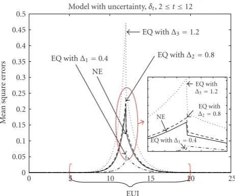
Figure 1compares the MSEs of NE-DFRHF (“NE”) with

three EQ-DFRHFs (“EQ”) with common horizon lengths Δ=Δi,i=1, 2, 3.

FromFigure 1we can observe that inside the EUI, the

NE-DFRHF is more accurate than the two EQ-DFRHFs with horizon lengthsΔ2 =0.8 andΔ3 = 1.2. However, the

NE-DFRHF is slightly worse than the EQ-NE-DFRHF with horizon lengthΔ1=0.4, that is,

PEQ22,t(Δ1)< PNE22,t< P22,EQt(Δ2)< P22,EQt(Δ3), t∈TEUI. (22)

Model with uncertainty,δt, 2≤t≤12

0 5 10 15 20 25

EUI 0

0.05 0.1 0.15 0.2 0.25 0.3 0.35 0.4 0.45 0.5

Me

an

sq

u

ar

e

er

ro

rs

NE

EQ withΔ3=1.2

EQ withΔ2=0.8

EQ withΔ1=0.4

NE

EQ with

Δ3=1.2

EQ with

Δ2=0.8

EQ withΔ1=0.4

Figure1: MSEs comparison between NE-DFRHF and three EQ-DFRHFsinsidethe EUI.

The reason for such a robust property (22) is to compensate for the given uncertainty δt, as the common

horizon lengthΔcomfor all local sensors (common memory

of LRHKFs) should be minimal. In this case, it is equal, as Δcom=Δ1=0.4.

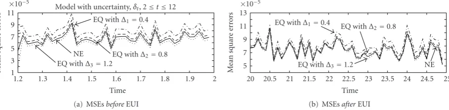
Figure 2, on the other hand, shows that outside the EUI,

the diﬀerences between the EQ-DFRHFs and NE-DFRHF are negligible. In this case, the EQ-DFRHF with the maximum common horizon lengthΔcom =Δ3 =1.2 is more accurate

than the NE-DFRHF, that is,

P22,EQt(Δ3)< P22,NEt< PEQ22,t(Δ2)< PEQ22,t(Δ1), t /∈TEUI. (23)

Figure 3 illustrates the time histories of the MSEs for

NE-DFRHF and the LRHKFs (LKF). This figure shows that inside the EUI, the MSE of NE-DFRHF is better than that of LRHKFs with the horizon lengthsΔ2=0.8 andΔ3=1.2, but

it is worse than the LRHKF withΔ1=0.4, that is,

PLKF

22,t(Δ1)< P22,NEt< PLKF22,t(Δ2)< P22,LKFt(Δ3), t∈TEUI.

(24)

Note, however, that outside the EUI the NE-DFRHF is better than all LRHKFs, as shown inFigure 4, that is,

PNE

22,t< P22,LKFt(Δ3)< P22,LKFt(Δ2)< P22,LKFt(Δ1), t /∈TEUI.

(25)

It should also be noted that the reduction of the horizon length to zero (Δi → 0) inside the uncertainty interval is

impossible due to the loss of sensor measurements (3). The problem in finding the optimal horizon lengthΔi for each

individual LRHKFs is quite complex.

Summarizing the simulation results provided in Figures 1–4, and using (22)–(25), we can conclude the following relations between MSEs inside/outside of the EUI:

PEQ22,t(Δ1)< P22,LKFt(Δ1)< PNE22,t< P

EQ

22,t(Δ2)< P22,LKFt(Δ2), t∈TEUI, P22,EQt(Δ3)< PNE22,t< P

EQ

22,t(Δ2)< P22,LKFt(Δ3)< PLKF22,t(Δ1), t /∈TEUI.

(5)

1.2 1.3 1.4 1.5 1.6 1.7 1.8 1.9 2 Time

1 3 5 7 9 11

×10−5

Me

an

sq

u

ar

e

er

ro

rs

NE EQ withΔ3=1.2

EQ withΔ2=0.8

EQ withΔ1=0.4

(a) MSEsbeforeEUI

20 20.5 21 21.5 22 22.5 23 23.5 24 24.5 25 Time

5 7 9 11 13

×10−5

Me

an

sq

u

ar

e

er

ro

rs

NE EQ withΔ3=1.2

EQ withΔ2=0.8

EQ withΔ1=0.4

(b) MSEsafterEUI

Figure2: MSEs comparison between NE-DFRHF and three EQ-DFRHFsbeforeandafterEUI.

0 5 10 15 20 25

EUI 0

0.05 0.1 0.15 0.2 0.25 0.3 0.35 0.4 0.45 0.5

Me

an

sq

u

ar

e

er

ro

rs

NE

LKF withΔ3=1.2

LKF withΔ2=0.8

LKF withΔ1=0.4

NE

LKF withΔ3=1.2

LKF withΔ2=0.8

LKF with

Δ1=0.4

Figure 3: MSEs comparison between NE-DFRHF and three LRHKFsinsidethe EUI.

Since, in actual situations, the uncertainty intervalT =

[a,b] is unknown in advance, the MSEs relation (26) proves NE-DFRHF to be the best choice among the other filters.

Example 6 (water tank mixing system). Consider a water tank system that accepts two diﬀerent water temperatures, while simultaneously throws oﬀthe mixed water [18]. This system is described by

˙

xt=

⎡ ⎢ ⎢ ⎢ ⎣

−0.0139 0 0

0 −0.0277 0

0 0.1667 −0.1667 + 0.1δt

⎤ ⎥ ⎥ ⎥ ⎦xt

+ ⎡ ⎢ ⎢ ⎢ ⎣ 1

1

1 ⎤ ⎥ ⎥ ⎥

⎦vt, t≥0,

(27)

where xt = [x1,t x2,t x3,t]T, x1,t is the water level, x2,t is

the water temperature,x3,tis the temperature of the sensor,

andvtis a white Gaussian noise. The initial values arex0 ∼ N(x0,P0),x0=[10 38 35]TandP0=diag[0.02 0.02 0.02].

Here, the system noise intensity Qt is 0.022 and the

time-varying uncertain model parameter is δt = sin(t) on the

interval 1≤t≤3:

δt=

⎧ ⎨ ⎩

sin(t), 1≤t≤3,

0, otherwise. (28)

The third coordinatex3,t, related to the sensor’s

tempera-ture of the water tank, is observable through a measurement model containing three identical local sensors: one primary sensor, with two reserves. In this case, we have

yt(i) =H(i)xt+w(ti), H(i)=

0 0 1T, i=1, 2, 3, (29)

where w(ti), i = 1, 2, 3, are white Gaussian noises with

intensitiesR(ti)=0.012,i=1, 2, 3.

We now present a model to show the robustness of the receding horizon filter against uncertainty [13]. In this example, we demonstrate the advantage of the receding horizon strategy using two filters: a distributed fusion receding horizon filter (see Section 3) and a distributed nonreceding horizon fusion filter (DNF) [17]. Three EQ-DFRHFs were designed for the diﬀerent common horizon lengthsΔ =0.4, 0.5, and 0.6. We focus on the MSEs of the third coordinatex3,t, called the sensor temperature, because

the time-varying uncertaintyδt from (27) appears only in

this coordinate:

P33,t=E

x3,t−x3,t 2, (30)

wherex3,t=xtEQ-DFRHForxDNFt .

Figure 5compares the MSEs of the EQ-DFRHFs (“EQ”)

for the horizon lengths of Δ = 0.4, 0.5 and 0.6. As can be observed in this figure, inside the time-interval TUI =

[1, 3], referred to as theUncertainty Interval (UI), all EQ-DFRHFs demonstrate better performance than DNF; this is in general agreement with the robustness of the receding horizon strategy. The MSEs of the nonreceding horizon filter DNF are remarkably larger than other EQ-DFRHFs. Also, the EQ-DFRHF with a horizon lengthΔ1=0.4 is more accurate

than the EQ-DFRHFs with horizon lengthsΔ2 = 0.5 and

Δ3=0.6, that is,

(6)

1.2 1.3 1.4 1.5 1.6 1.7 1.8 1.9 2 Time

4 6 8 10 12×

10−5

Me

an

sq

u

ar

e

er

ro

rs

NE LKF withΔ3=1.2

LKF withΔ2=0.8

LKF withΔ1=0.4

(a) MSEsbeforeEUI

20 20.5 21 21.5 22 22.5 23 23.5 24 24.5 25 Time

4 6 8 10 12

×10−5

Me

an

sq

u

ar

e

er

ro

rs

NE LKF withΔ3=1.2

LKF withΔ2=0.8

LKF withΔ1=0.4

(b) MSEsafterEUI

Figure4: MSEs comparison between NE-DFRHF and three LRHKFsbeforeandafterEUI.

0 1 2 3 4 5 6

UI 0

0.5 1 1.5 2 2.5 3

Me

an

sq

u

ar

e

er

ro

rs DNF

EQ withΔ3=0.6

EQ withΔ2=0.5

EQ withΔ1=0.4

Figure5: MSEs comparison between DNF and three EQ-DFRHFs.

On the other hand, outside the UI the diﬀerences between the DFRHFs are negligible, though the EQ-DFRHF with a maximum common horizon length ofΔcom=

Δ3=0.6 is more accurate than other EQ-DFRHFs, that is,

P33,EQt(Δ3)< P33,EQt(Δ2)< P33,EQt(Δ1), t /∈TUI. (32)

Summarizing the simulation results in Figure 5, EQ-DFRHF has a parallel structure and allows parallel processing of observations, thereby making it more reliable than the others since the remaining faultless sensors can continue the fusion estimation if some sensors become faulty. Moreover, EQ-DFRHF can produce high-quality results in a real-time processing environment.

5. Conclusions

In this paper, we proposed a new distributed receding horizon filter for a set of local sensors with nonequal horizon lengths. Also, we derived the key diﬀerential equations for determining the local cross-covariances between LRHKFs with the diﬀerent horizon lengths.

Furthermore, it was found that NE-DFRHF can com-plement for robustness and accuracy when a common time interval containing all sensor data is lacking. Subsequent

simulation results and comparisons between NE-DFRHF and other EQ-DFRHFs and LRHKFs verify the estimation accuracy and robustness of the proposed filter.

Appendix

Derivation of

(

13 )

–

(

17 )

Local filtering errorse(si)andes(j),i /=j satisfy the following

equations:

˙

e(i)

s =Fs(i)e(si)−Ks(i)ws(i)+Gsvs, s∈[t−Δi,t],

˙

es(j)=Fs(j)e(sj)−Ks(j)ws(j)+Gsvs, s∈

t−Δj,t

.

(A.1)

Next, without losing generality, let us assume that

Δi<Δj or t−Δi> t−Δj. (A.2)

Then, on the common time-intervals∈[t−Δi,t], (A.1) can

be rewritten in the following form:

˙

Es(i j)def=

⎡ ⎣e˙

(i)

s

˙

es(j)

⎤ ⎦₌_A(i j)

s E

(i j)

s +B(si j)η

(i j)

s , s∈[t−Δi,t],

A(si j)=

⎡ ⎣F

(i)

s 0

0 Fs(j)

⎤

⎦, B(si j)=

⎡ ⎣−K

(i)

s Gs 0

0 Gs −Ks(j)

⎤ ⎦_,

ηs(i j)=

w(si)T vsT w

(j)T

s

T

, η(si j)∼N

0,Q(sη)

,

Qs(η)=diag

R(si) Qs R(sj)

(A.3)

with the special horizon initial conditions:

E(s=i j)t−Δi = ⎡ ⎢ ⎣e

(i)

s=t−Δi

es(=j)t−Δj ⎤ ⎥ ⎦=

⎡

⎣xt−Δi−x(t−i)Δi

xt−Δi−x(t−j)Δi ⎤ ⎦(6)

=

⎡

⎣xt−Δi−mt−Δi xt−Δi−x(

j)

t−Δi ⎤ ⎦_,

mt−Δj =E

xt−Δj

.

(7)

Application of the Lyapunov equation to the model (A.3) yields the following diﬀerential equation for the cross-covariance Cs(i j) = cov{Es(i j),E(si j)} on the common

time-interval:

˙

C(si j)=A(si j)C

(i j)

s +C(si j)A(i j)

T

s +B

(i j)

s Q

(η)

s B(i j)

T

s ,

C(si j)=

⎡ ⎢ ⎣

coves(i),e(si)

cove(si),e(sj)

cove(sj),e(sj)

⎤ ⎥ ⎦ = ⎡ ⎢ ⎣P

(ii)

s P(si j)

P(i j)

T

s P(sj j)

⎤ ⎥ ⎦.

(A.5)

Substituting the matricesA(si j),B

(i j)

s , andQ

(η)

s into (A.5),

we obtain the following equation for the cross-covariance

Ps(i j):

˙

P(si j)=F(si)P

(i j)

s +Ps(i j)F(j)

T

s +GsQsGTs, s∈[t−Δi,t]

(A.6)

with the initial condition:

Ps(=i jt)−Δi=cov

e(t−i)Δi,e

(j)

t−Δi _(A_.₄₎

= Pt−Δi−cov

xt−Δi,x

(j)

t−Δi

.

(A.7)

To determine the covariance cov{xt−Δi,x

(j)

t−Δi}in (A.7), let us consider a set of stochastic equations for the statexτand its

estimatexτ(j)on the remain time-intervalτ∈[t−Δj,t−Δi].

From (1) and (5) we obtain

˙

Zτ(j)def=

⎡ ⎣ x˙τ

˙_x(j)

τ

⎤ ⎦₌_A(j)

τ Zτ(j)+Bτ(j)ξτ(j), τ∈

t−Δj,t−Δi

(A.8)

with the initial condition:

Zτ(=j)t−Δj = ⎡ ⎣xt−Δj

x(t−j)Δj

⎤ ⎦(A.4)

=

⎡ ⎣xt−Δj

mt−Δj ⎤

⎦, (A.9)

where ξτ(j) = [vτT w

(j)T

τ ] T

is a white Gaussian noise with intensity matrixQ(τj)=diag[Qτ R(τj)].

Then, the covariance of vectorZτ(j)

Dτ(j)def=cov

Zτ(j),Z(τj)

=

⎡ ⎢

⎣cov{xτ,xτ} cov

xτ,x

(j)

τ

covxτ(j),xτ

covx(τj),x(τj)

⎤ ⎥ ⎦,

τ∈t−Δj,t−Δi

(A.10)

is described by the Lyapunov equation for the model (A.8):

˙

Dτ(j)=A(τj)Dτ(j)+D(τj)A(j)

T

τ +B(τj)Q(τj)B(j)

T

τ ,

τ ∈t−Δj, t−Δi

.

(A.11)

Since the second component of the initial vectorZτ(=j)t−Δj is nonrandom (xt(−j)Δj = mt−Δj), the structure of the initial covarianceD(τj=)t−Δjcan then take the special form:

D(τj=)t−Δj = ⎡ ⎣cov

xt−Δj,xt−Δj 0 0 0 ⎤ ⎦₌ ⎡ ⎣Pt−Δj 0

0 0 ⎤

⎦, (A.12)

where the nonzero elementPt−Δj in (A.7) and (A.12) repre-sents the covariance of the statext−Δj, which is determined by the Lyapunov equation (7).

This completes the proof ofTheorem 2.

Acknowledgments

This work was supported by ADD (contract no. 912176201) and the BK21 program partly at Gwangju Institute of Science and Technology.

References

[1] Y. Bar-Shalom and X. R. Li,Multitarget-Multisensor Tracking: Principles and Techniques, YBS Publishing, Storrs, Conn, USA, 1995.

[2] Y. M. Zhu,Multisensor Decision and Estimation Fusion, Kluwer Academic Publishers, Boston, Mass, USA, 2003.

[3] S.-L. Sun, “Multi-sensor optimal information fusion Kalman filters with applications,”Aerospace Science and Technology, vol. 8, no. 1, pp. 57–62, 2004.

[4] S.-L. Sun and Z.-L. Deng, “Multi-sensor optimal information fusion Kalman filter,” Automatica, vol. 40, no. 6, pp. 1017– 1023, 2004.

[5] Yaakov. Bar-Shalom and L. Campo, “The eﬀect of the common process noise on the two-sensor fused-track covariance,”IEEE Transactions on Aerospace and Electronic Systems, vol. 22, no. 11, pp. 803–805, 1986.

[6] H. R. Hashemipour, S. Roy, and A. J. Laub, “Decentralized structures for parallel Kalman filtering,”IEEE Transactions on Automatic Control, vol. 33, no. 1, pp. 88–94, 1988.

[7] T. M. Berg and H. F. Durrant-Whyte, “General decentralized Kalman filters,” inProceedings of the American Control Confer-ence (ACC ’94), vol. 2, pp. 2273–2274, Baltimore, Md, USA, 1994.

[8] Y. Zhu, Z. You, J. Zhao, K. Zhang, and X. R. Li, “The optimality for the distributed Kalman filtering fusion with feedback,” Automatica, vol. 37, no. 9, pp. 1489–1493, 2001.

[9] X. R. Li, Y. Zhu, J. Wang, and C. Han, “Optimal linear estima-tion fusion—part I: unified fusion rules,”IEEE Transactions on Information Theory, vol. 49, no. 9, pp. 2192–2208, 2003. [10] J. Zhou, Y. Zhu, Z. You, and E. Song, “An eﬃcient algorithm

for optimal linear estimation fusion in distributed multi-sensory systems,” IEEE Transactions on Systems, Man, and Cybernetics, vol. 36, no. 5, pp. 1000–1009, 2006.

[11] A. H. Jazwinski, Stochastic Processes and Filtering Theory, Academic Press, New York, NY, USA, 1970.

[12] W. H. Kwon, K. S. Lee, and O. K. Kwon, “Optimal FIR filters for time-varying state-space models,” IEEE Transactions on Aerospace and Electronic Systems, vol. 26, no. 6, pp. 1011–1021, 1990.

(8)

Transactions on Automatic Control, vol. 44, no. 11, pp. 2115– 2120, 1999.

[14] D. Y. Kim and V. Shin, “Optimal receding horizon filter for continuous-time nonlinear stochastic systems,” inProceedings of the 6th WSEAS International Conference on Signal Processing (ICSP ’08), pp. 112–116, Dallas, Tex, USA, 2007.

[15] D. Y. Kim and V. Shin, “An optimal receding horizon FIR filter for continuous-time linear systems,” in Proceedings of the 18th SICE-ICASE International Joint Conferences (SICE-ICCAS ’06), pp. 263–265, Busan, South Korea, 2006.

[16] I. Y. Song, D. Y. Kim, and V. Shin, “Distributed receding hori-zon filtering for linear multisensor continuous-time systems,” inProceedings of the 10th IASTED International Conference on Signal and Image Processing (SIP ’08), pp. 238–242, Kailua-Kona, Hawaii, USA, 2008.

[17] V. Shin, Y. Lee, and T.-S. Choi, “Generalized Millman’s formula and its application for estimation problems,”Signal Processing, vol. 86, no. 2, pp. 257–266, 2006.