Volume 2008, Article ID 216453,12pages doi:10.1155/2008/216453
Research Article
Boosted and Linked Mixtures of HMMs for
Brain-Machine Interfaces
Shalom Darmanjian and Jose C. Principe
Department of Electrical and Computer Engineering, University of Florida, Gainesville, FL 32611, USA
Correspondence should be addressed to Jose C. Principe,[email protected]
Received 9 October 2007; Accepted 26 February 2008
Recommended by An´ıbal Figueiras-Vidal
We propose two algorithms that decompose the joint likelihood of observing multidimensional neural input data into marginal likelihoods. The first algorithm, boosted mixtures of hidden Markov chains (BMs-HMM), applies techniques from boosting to create implicit hierarchic dependencies between these marginal subspaces. The second algorithm, linked mixtures of hidden Markov chains (LMs-HMM), uses a graphical modeling framework to explicitly create the hierarchic dependencies between these marginal subspaces. Our results show that these algorithms are very simple to train and computationally efficient, while also reducing the input dimensionality for brain-machine interfaces (BMIs).
Copyright © 2008 S. Darmanjian and J. C. Principe. This is an open access article distributed under the Creative Commons Attribution License, which permits unrestricted use, distribution, and reproduction in any medium, provided the original work is properly cited.
1. INTRODUCTION
The field of brain-machine interfaces (BMIs) is devoted to accomplishing the goal of one day restoring paralyzed patients mobility by directly connecting their brain to a machine. A majority of developments in this field have centered around linear and nonlinear models that map neural firing patterns of an animal to a robotic prosthetic [1–3]. Usually, in this type of experiment, a primate or rat engages in a movement task as neural data is recorded from their cortex (as well as the kinematic information). Once a prediction model has been trained with the trajectory/neural data, only neural data is used to control a robotic arm in real-time [2,3].
As a result of the above-mentioned experiments, our group established that when multiple feed-forward predic-tion models map discrete porpredic-tions of the neural data to respective portions of the continuous trajectory, the overall trajectory reconstruction is improved [4,5]. The classifier that is responsible for switching between these different feed-forward models is the main focus of this paper (seeFigure 1
for system overview).
The previous switching classifier was an ensemble method that incorporated multiple independent experts. These experts were single neural-channel HMM chains that
formed an independently coupled hidden Markov model (IC-HMM) [5]. Since it is unlikely that the independence assumption applies to all of the neurons, finding dependen-cies between some of the neurons, could prove beneficial for final kinematic reconstruction or other biologically-inspired modeling. Additionally, one limitation of this algorithm is that as more neurons are sampled from the brain (as is the current trend for BMIs), the number of independent models could grow to an unmanageable level [6]. Although the ICHMM is still computationally more efficient than using a model that has full dependencies, like the coupled hidden Markov model (CHMM), it is still desirable that the input dimensionality be reduced to avoid this pitfall.
Pre-processing spike detection/sorting
Feed forward models computing 3D trajectory
Switching classifier selects corresponding forward model
Robotic arm real-time control
Acquire multichannel neural data
O1
1
O1
2
O1
T O2
T
O2
1
O2
2 S2
1 S2
2
S2
T
S1
T
T1
T2
S1
1
S1
2
M1 M2
· · ·
· · ·
··· ···
Ti m e
Neural channels
Figure1: BMI overview.
We then move from this method, which only implicitly exploits the dependencies between the neurons, to a more formal graphical model structure which explicitly models dependencies between neurons. We call this model linked mixture of hidden Markov chains (LM-HMM). Borrowing ideas from the BM-HMM, we show how this semisupervised model explicitly exploits the dependencies between neurons (if they exist).
The development and evaluation of the BM-HMM and LM-HMM serve as the core of this paper and directs the following organization. First, we discuss our motivation and technique for the BM-HMM. Second, we develop the theory for the LM-HMM and explain how it relates to the BM-HMM. Third, we compare results of the new models to our previous models, as well as present some possible interpretation of the results. Finally, we suggest areas of future work.
2. MODELING NEURAL DATA FOR BRAIN-MACHINE INTERFACES
2.1. Experimental animal data
Neural action potentials from two different animal experi-ments are used to train and test the models in this paper. In the first experiment, neural data was recorded from an owl monkey’s cortex as it performed a food reaching task. Specifically, multiple implanted microwire arrays recorded this data from 104 neural cells in the following cortical areas: posterior parietal cortex (PP), left and right primary motor cortex (M1), and dorsal premotor cortex (PMd). Concurrently with the neural data recording, the 3D hand position was recorded as the monkey made three repeated movements: rest to food, food to mouth, and mouth to rest [1,5].
In the second experiment, a male Sprague-Dawley rat performed a go, no-go lever pressing task as neural data was recorded. This dataset contains 16 neural cells that were collected with microwire arrays implanted in the forelimb region of the left primary cortex (M1) [7]. Subsequently, the data was spike-detected and spike-sorted using thresholds and template matching [7]. The lever presses were recorded simultaneously with the neural activity. The beginning of each trial was signaled to the rat by an LED indicating when to press the lever in order to receive a reward [7].
The data sets resulting from the above experiments were segmented into movement and rest classes for modeling. For the monkey data, all angular velocities greater than 4 mm/s are labeled as part of the movement class. Included in this movement class are the times when the monkey momentarily holds its arm during a reach for food or its mouth [5,8]. For the rat experiments, since there is no information about the rat moving around the cage (or grooming), only the lever press is included as part of the movement class [7].
For both experiments, the neural data is binned into 100-millisecond counts, which is consistent with the neural science community [8,9]. Consequently, the movement data is down-sampled to match the 10 Hz neural bin counts. The time recording for the monkey experiment corresponds to a dataset of 23000×104 time bins. For the rat experiment, the dataset consists of 13000×16 time bins [1,7].
2.2. Motivation
neurons exhibit nonstationary behavior [11]. Our group’s own work has shown that modeling this data as a single multivariate process is not the most appropriate [4]. It is also inappropriate to model all of the channels independently since there is a possibility of dependencies between some of the neurons.
From a machine learning perspective, modeling of the observed and hidden neural information can be accom-plished with observable and hidden random processes that are interacting with each other in some unknown way. To achieve this, we make the assumption that each neuron’s output is an observable random process that is affected by hidden information. Since the experiment does not pro-vide detailed biological information about the interactions between the sampled neurons, we use hidden variables to model these hidden interactions [9,12]. We further assume that this compositional representation of the interacting processes occurs through space and time (i.e., between neurons at different times).
We also differ from other work in the BMI field by not taking the traditional regression approach of mapping the neural data directly to the patient hand kinematics with a conventional linear/nonlinear model [10]. Since the final BMI paradigm will not include desired kinematic information from paraplegics, we use generative models to explain the observable neural data. From these generative models, we divide the input space into regions that we call “motion primitives.” These structures have been loosely touched upon in other work [13,14]. The basic idea is that kinematic information or neural data can be decomposed into these “motion primitives” similar to phonemes in speech processing. In speech processing, graphical models (specifically HMMs) are the leading technology because they are able to capture very well the piecewise nonstationarity of speech [15, 16]. Since speech production is ultimately a motor function, graphical models can potentially also be useful for motor BMIs (also nonstationary) [11, 15]. By using smaller simpler components, more complicated arm kinematics can be constructed through the combination of these simple structures.
The ultimate goal is to decipher these underlying struc-tures so that the model may one day be decoupled from the desired kinematics (for unsupervised modeling). It is our current goal to determine these underlying structures through a supervised mode in order to later exploit them in an unsupervised mode.
3. BOOSTED MIXTURES OF HMM CHAINS
3.1. Related work
With IC-HMMs, each neural channel is modeled with a hidden and observable random process (i.e., an HMM chain) [5]. Each neural channel HMM in the IC-HMM is computed independently. To calculate the log likelihood for the IC-HMM (Figure 2) we use
logP(O|S,Θ)= N
i=1
logPOi|Si,Θi, (1)
O11
O1
2
O1
T O1T
O1
1
O1
2
S1
1
S1
2
S1
T
S1
T
S11
S1
2
· · ·
··· ···
Ti m
e
Neural channels Figure2: IC-HMM graphical model.
where Θi is the set of all the parameters for the model of a particular neural channel (where i = 1,. . .,N neural channels). Given that, Oi = (Oi
1,Oi2,. . .,OiT) is a sequence
of discrete binned neural firings andSi=(Si
1,Si2,. . .,SiT)
rep-resents the sequence of discrete hidden states or variables (of lengthT), this joint probability can be further decomposed into
logP(O|S,Θ)= N
i=1
logPSi1
+ T
t=1
logPOit|Sit,Θi
+ T
t=2
logPSi
t|Sit−1,Θi
.
(2)
FromFigure 2and (2), we see that the observable var-iables are IID and the hidden state sequence is Markovian (which is the classical HMM formulation). Essentially, the IC-HMM decomposes the multivariate input into the independent marginals so that only the likelihoods of the individual neurons are needed for the final calculation [5].
In order to move beyond the IC-HMM and exploit the complimentary information provided by the independent HMM chains, we first look to boosting. Boosting is a technique that creates different training distributions from an initial input distribution so that a set of weak classifiers is generated [17, 18]. The generated classifiers then form an ensemble vote for the current data example. It has been shown that these hierarchic combinations of classifiers achieve lower error rates than the individual base classifiers [17,18].
Adaboost is the most widely used algorithm to evolve from boosting methods [19]. This algorithm sequentially generates weak classifiers based on weighted training exam-ples. Essentially, the initial distribution of training examples is resampled each round (based on the distribution of the weights Wi) in order to train the next classifier up to R rounds [19]. The training examples that fail to be classified on a particular round receive an increased weighting so that the subsequent classifiers are more likely to be trained on these hard examples. With the initial values of the weights beingWi = 1/n, fori = 1,. . .,N samples, the update for each weight is
Wi←−
Wiexp
αr·1(y /=fr(x))
Zr
where αr are the external weights for eachrth expert that has been trained for the rth round which act very similar to priors for the respective experts. Additionally, Zr is a normalization factor in order to make the weights Wi a distribution. Concurrent to the weights Wi for training examples, each αr is updated so that it can be used in a final ensemble vote (which is a linear combination of theαr weights and the hypothesis of each expert):
αr=log
1−errr
errr , (4)
where
errr= N
i=1
Wi
yi=/h(xi) (5)
and the final ensemble output becomes
H(x)=sign
R
r=1
αrfr(x)
. (6)
The success of boosting has been attributed to the distribution of the “margins” of the training examples [17]. For further details on Adaboost or boosting with respect to the margin and relationships to support vector machines, see Schapier et al.
With respect to improving IC-HMM, Adaboost offers a promising way to implicitly find dependencies among the channels through the process of boosting classifiers during training. In our case, Adaboost is applied differently to the multidimensional neural data as explained in the next section.
3.2. Modeling framework
BMI data imposes specific constraints that require mod-ifications to the standard procedures. First, our data is high dimensional (104 channels) and the importance of each channel to the mapping can be very different and is unknown. Second, the classes have markedly different prior probabilities. Third, the computational practicality of using thousands of experts to generate a decision is infeasible for hundreds of neural channels. Our approach uses Adaboost as a way to select multichannel experts that contribute the most information in the training set. Although the algorithm starts out with parallel training for the independent experts, gradually a winning expert is chosen for each hierarchic level to combine later into the ensemble. Since each level is formed in an unsupervised way, this algorithm is a hybrid between supervised and unsupervised learning, following a process similar to the mixture of experts framework [20].
Our first major departure from Adaboost results from how the ensemble is generated. Instead of forming one expert at a time, the M independent HMM chains are trained in parallel using the Baum-Welch formulation [21]. As explained, this splits the joint likelihood into marginals so that independent processes are working in simpler subspaces [5]. A ranking is then performed and a winner is chosen
based on the classification performance for the current distribution of input examples. Specifically, the winner that minimizes the error with respect to the distribution of samples is chosen. To find the minimal error, we differ from Adaboost and use an Euclidean distance for the classes to avoid biasing class assignments (since classes may not have equal priors) [5]. Next, the remaining experts are trained within their respective subspace but relative to the errors of the previous winner. Finally, the Wi are used to select the next distribution of examples for the remaining experts. Similar to Adaboost, the remaining experts are trained on the hard examples from different subspaces. In turn, a hierarchic structure is formed as the winning experts affect the training on the local subspaces for the subsequent experts. During this process, they are implicitly modeling the dependencies among the channels.
As explained earlier, Adaboost uses αm’s as external weights to the classifiers as opposed to the Wi’s which weight the training examples. Our computation of theαm’s is the second major departure from Adaboost since we use a mixture of experts formulation for the external weights or mixture coefficients. To find the mixture coefficients for the local classifiers, we look to the boosted mixture of experts (BME) [22]. With BME, improved performance is gained through the use of a confidence measure for the individual experts [22]. Although many different confidence measures exist, the majority use a scalar function of the expert’s output which is then used as a static gating function or mixture coefficient [20,22]. Our algorithm uses a simple measure for each expert based on theL2-Norm of the class errors (instead of the one outlined in (4)):
αm=1−
err2
M+ err2R, (7)
where errM and errR are the respective errors of the two classes in our problem, move and rest (which could generalize to more classes). We useβmto substitute for the normal Adaboost formulation ofαm (4) to update theWi’s in (3).
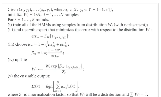
Since there is a condition placed during the boosting phase to discard experts with less than 50% classification, negative alphas will not occur [19]. Notice that as the errors between the two classes are smaller, the weights for the experts become larger. We present the proposed Adaboost training algorithm for BM-HMM (seeAlgorithm 1).
The criterion for stopping is based on two conditions. The first stopping condition occurs, if the chosen experts are performing less than 50% classification. The second stopping condition occurs if the cross-validation set shows an increase in error or a plateau in performance for a significant number of rounds.
Given (x1,y1),. . ., (xn,yn), wherexi∈X, yi∈Y= {−1, +1}, initializeWi=1/N, i=1,. . .,Nsamples.
Forr=1,. . .,Rrounds,
(i) train all of the HMMs using samples from distributionWi(with replacement); (ii) find themth expert that minimizes the error with respect to the distributionWi:
errm=EW
1(y /=fm(x)) ;
(iii) chooseαm=1−
err2
M+ err2R:
βm=log 1−errm
errm ; (iv) update
Wi←−
Wiexpβm·1(y /=fm(x)) Zr
;
(v) the ensemble output:
H(x)=sign
M
m=1 αmfm(x)
,
whereZris a normalization factor so thatWiwill be a distribution and
iWi=1.
Algorithm1
O11
O1
2
O1
T O2T
O21
O2
2
S2
1
S2
2
S2
T
S1
T
T1
T2
S1
1
S1
2
M1 M2
· · ·
· · ·
··· ···
Ti m
e
Neural channels Figure3: LM-HMM graphical model.
In the next section, we slightly increase the complexity of the BM-HMM to explicitly model dependencies between the neurons.
4. LINKED MIXTURES OF HMM CHAINS
4.1. Modeling framework
Let Z represents the set of variables (both hidden and observed) included in the probabilistic model. A graphical model (or Bayesian network) representation can then be used to provide insight into the probability distributions over
Zencoded in a graph structure [23]. With this type of repre-sentation, edges of the graph represent direct dependencies between variables. Conversely, and more importantly, the absence of an edge allows the assumption of conditional independence between variables. Ultimately, these condi-tional independencies allow a more complicated multivariate distribution to be decomposed (or factorized) into simple and tractable distributions [23].
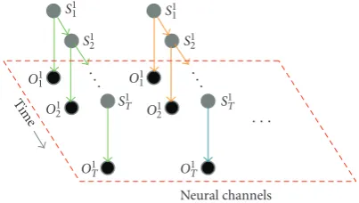
Since there is a variety of graphical model representations that decomposes the joint probability of the hidden and observed variables inZ, choosing the best approximation is overwhelming. To move beyond the IC-HMM and implicit dependencies in the BM-HMM, we establish another layer of hidden or latent variables to link and express the spatial dependencies between the lower level HMM structures (Figure 3), thus creating a clique tree structure T (since there are cycles), where hierarchic links exist between neural channels.
The log likelihood of the dynamic neural firings from all of the neurons for this structure (Figure 3) is
logP(O|S,M,Θ)=logPM1+
N
i=2
logPMi|Mi−1,Θ
+ N
i=1
T
t=1
logPOi t|Sit,Θi
+ T
t=1
logPSit|Sti−1,Mi,Θi
,
(8)
where the dependency between the tree cliques are repre-sented by a hidden variableMin the second layer:
PMi|Mi−1,Θi (9)
and the hidden state sequenceSalso has a dependency on the hidden variableMin the second layer:
PSi
t|Sit−1,Mi,Θi
. (10)
second layer hidden variable Mi as well as the subgraphs of the other neural channels Tj (wherei /=j). The hidden variableM in the second layer of (8) can be interpreted as a mixture variable (when excluding the hierarchic links).
The LM-HMM implements a middle ground between making an independence assumption and a full dependence assumption. Since we are adding a layer of hidden variables, we are incurring a computational cost. The next section will show that we can make an approximation to ease compu-tational costs but still bring in the richness of modeling the interrelationships between neurons.
4.2. Training with expectation maximization (EM)
Although using EM with graphical models gives us insight into probability distributions over our observed and hidden variables, some probabilities of interest are intractable to compute. Instead of using brute force methods to evaluate such probabilities, conditional independencies represented in the graphical model can be exploited. Often, approx-imations like Gibbs sampling, variational methods, and mean field approximations are applied in order to make the problem tractable or computationally efficient [23,24].
For our model, we use a mean field approximation to allow interactions associated with tractable substructures to be taken into account [24]. The basic idea is to associate with the intractable distribution a simplified distribution that retains certain terms of the original distribution while neglecting others, replacing them with parameters ui that we will refer to as “variational parameters.” Graphically, the method can be viewed as deleting edges from the original graph until a forest of tractable structures is obtained. Edges that remain in the simplified graph correspond to terms that are retained in the original distribution and edges that are deleted correspond to variation parameters [24,25].
We make approximations when finding the expectation of (8). In particular, we will first approximate P(Sit | Sit−1, Mi,Θi) by treatingMias independent fromSmaking condi-tional probability equal to the familiarP(Sit |Sit−1,Θi). Two
important features can be seen in this type of approximation. First, we have decoupled the simple lower-level HMM chains from the higher-levelMi variables. Second,Mican now be regarded as a linked mixture variable for the HMM chains sinceP(Mi|Mi−1,Θi) which we will address later [20].
Because the lower-level HMMs have been decoupled, we are able to use the Baum-Welch formulation to compute some of the calculations in the E-step, leaving estimation of the variational parameter for later. As a result, we can calculate the forward pass:
Estep
αj(t)=P
O1=o1,. . .,Ot=ot,St= j|Θ
. (11)
We can calculate this quantity recursively by setting
αj(1)=πjbj
o1
,
αk(t+ 1)=
N
j=1
αj(t)ajk
bk(ot+1).
(12)
The well-known backward procedure is similar:
βj(t)=P
Ot+1=ot+1,. . .,OT =oT |St= j,Θ
, (13)
this computes the probability of the ending partial sequence
ot+1,. . .,oTgiven the start at statejat timet. Recursively, we
can defineβj(t) as
βj(T)=1,
βj(t)=
N
k=1
ajkbk
ot+1
βk(t+ 1).
(14)
Additionally, theajk andbj(ot) matrices are the transi-tion and emission matrices defined for the model which are updated in the M-step. Continuing in the E-step, we will rearrange posteriors in terms of the forward and backward variables. Let
γj(t)=P
St=j|O,Θ
(15)
which is the posterior distribution. We can rearrange the equations to quantities so we have
PSt =j|O,Θ
=P
O,St=j|Θ
P(O|S,Θ) =
PO,St=j|Θ
N
k=1P
O,St=k|Θ
(16)
and now with the conditional independencies we can define the posterior in terms ofα’s andβ’s:
γj(t)=
αj(t)βj(t)
N
k=1αk(t)βk(t)
. (17)
We also define
ξjk(t)=P
St=j,St+1=k|O,Θ
(18)
which can be expanded as
ξjk(t)=P
St=j,St+1=k,O|Θ
P(O|S,Θ)
= αj(t)ajkbk
ot+1
βk(t+ 1)
N
j=1
N
k=1αj(t)ajkbk
ot+1
βk(t+ 1)
.
(19)
TheM-step departs from the Baum-Welch formulation and introduces the variational parameter [24]. Specifically, theM-step involves the update of the parametersπj,ajk,bL (we will saveuifor later):
Mstep
πi
j=
I
i=1uiγ1i(j)
I i=1ui
,
ai
jk=
I
i=1ui
T−1
t=1ξti(j,k)
I
i=1ui
T−1
t=1γit(j) ,
bi
j(L)=
I
i=1ui
T
t=1δot,vLγ
i t(j)
I
i=1ui
T
t=1γit(j)
.
There are two issues left to resolve. First, how can the variational parameter be estimated and maximized given the dependencies. Second, if experimentally it is not known which neurons are affecting other neurons (if at all), how can the dependencies between neurons be defined in the model.
4.3. Updating variational parameter via importance sampling
While still working within the EM framework, we treat the variational parametersuias mixture variables generated by the ith HMM each having a prior probability of pi. We want to estimate the set of parameters that maximize the likelihood function [25–27]:
n
z=1
I
i=1
piPOzi|Si,Θi. (21)
Given the set of sequences and current estimates of the parameters, theE-step consists of computing the conditional expectation of hidden variableM:
uzi=E
Mi|Mi−1,Ozi|Θi =PrMi=1|Mi−1=1,Ozi,Θi .
(22)
The problem with this conditional expectation is the dependency onMi−1. SinceMi−1is independent fromOiand Θi, we can decompose this into
uzi=E
Mi|Ozi,Θi EMi|Mi−1 . (23)
The first term, a well-known expectation for mixture of experts, is calculated by using Bayes rule and the priori probability thatM=1:
EMi|Oi,Θi =PrMi=1|Oi,Θi = piP
Oi|Si,Θi
I
i=1piP
Oi|Si,Θi.
(24)
Since the integration for the second term is much harder to compute, we look to an integration approximation that will maintain the dependencies. Importance sampling is a well-known method that is capable of approximating the integration with a lower variance than Monte-Carlo integration [28]. We can approximate the integration with
EMi|Mi−1 =1
n
n
z=1
POzi|Si,Θi
POz(i−1)|Si−1,Θi−1, (25)
where the n samples have been drawn from the proposal distributionP(Ozi−1 |Si−1,Θ). For the estimation ofu
i, we need to combine the two terms:
uzi= p
iPOzi|Si,Θi
I
i=1piP
Ozi|Si,Θi
n
z=1
POzi|Si,Θi
nPOz(i−1)|Si−1,Θi−1.
(26)
To compute theM-step,
pi=
n
z=1uzi
I
i=1
n
z=1uzi =
n
z=1uzi
n . (27)
Table1: Classification results (BM-HMM selected channels).
Model Channels no. % correct
With monkey data
IC-HMM 104 92.4%
IC-HMM 9 87.1%
BM-HMM 9 92.0%
Linear 104 88.3%
Linear 9 86.9%
With rat data
IC-HMM 16 62.5%
IC-HMM 6 58.3%
BM-HMM 6 64.0%
Linear 16 61.8%
Linear 6 56.9%
Table2: Classification results (random LM-HMM selected chan-nels).
Model Channels no. % correct
With monkey data
IC-HMM 104 92.4%
IC-HMM 9 89.5%
LM-HMM 9 92.1%
Linear 104 88.3%
Linear 9 87.8%
With rat data
IC-HMM 16 62.5%
IC-HMM 6 56.5%
LM-HMM 6 62.3%
Linear 16 61.8%
Linear 6 55.2%
Borrowing from the competitive nature of the BM-HMM, we choose winners based on the same criterion of minimizing the Euclidean distance for the classes for the LM-HMM.
5. EXPERIMENTAL RESULTS
5.1. Quantitive results
In this section, we first show the results of our model on the two animal experiments. Next, we illustrate the effects of the algorithm by comparing the BM-HMM and LM-HMM chains to the IC-HMM chains. The BM-HMM and LM-HMM chains are ranked in order of the rounds, while the IC-HMM chains are ranked from the best to worst in terms of the individual chain’s ability to classify. We conclude with an analysis of the methods by randomly selecting the chains for the LM-HMM and BM-HMM to understand if dependencies are being captured.
Table3: Classification results (random BM-HMM selected chan-nels).
Model channels no. % correct
With monkey data
IC-HMM 104 92.4%
IC-HMM 9 69.1%
BM-HMM 9 69.4%
Linear 104 88.3%
Linear 9 68.1%
With rat data
IC-HMM 16 62.5%
IC-HMM 6 56.5%
BM-HMM 6 56.9%
Linear 16 61.8%
Linear 6 55.1%
Table4: Classification results (random LM-HMM selected chan-nels).
Model channels no. % correct
With monkey data
IC-HMM 104 92.4%
IC-HMM 9 63.5%
LM-HMM 9 65.4%
Linear 104 88.3%
Linear 9 63.2%
With rat data
IC-HMM 16 62.5%
IC-HMM 6 55.4%
LM-HMM 6 54.3%
Linear 16 61.8%
Linear 6 54.8%
and a simple linear classifier created by a regression model followed by a threshold [5]. For the HMMs, we use three hidden states and an observation sequence lengthT = 10, which corresponds to one second of data (given the 100-millisecond bins). These choices were based on previous efforts to optimize performance [4]. For the linear classifier, a Wiener filter with a 10-tap delay (that corresponds to one second of data) is used. These parameters and thresholds were also chosen based on previous work [4, 13]. The classification results are determined on each data point in the training set. Cross-validation sets, Monte-Carlo runs, leave-K-out methodologies are also employed to make sure that our results are general.
As seen in Tables1,2,3, and4, the correct classification percentage is much higher for the monkey data than the rat data. This is explained primarily by the experimental conditions. Since the rat experiment is not as controlled as the monkey experiment, the rat dataset is much noisier. In particular, as the rat moves around the cage there are many training and testing samples labeled as nonmovement,
0 0.1 0.2 0.3 0.4 0.5 0.6 0.7 0.8 0.9 1
Er
ro
r
(%)
0 20 40 60 80 100 120
Number of experts IC-HMM
BM-HMM
LM-HMM
Figure4: Monkey expert adding experiment.
when the animal is actually moving (only lever presses are counted as movement in this setup). This explains the much lower performance on the rat data. Also, fewer neural channels were collected from the rat than the monkey [1,7]. Apart from this difference, the same trends are seen in both datasets.
To give a fair comparison between the methods, the same neural channels that were chosen by the BM-HMM are used with the linear model and the IC-HMM. For the LM-HMM, a different set of neurons (although some overlap the BM-HMM) was selected based on the algorithm, but the number of final channels were kept the same. As compared in Tables1 and2, the BM-HMM and LM-HMM perform on par with the IC-HMM, but with the added benefit of dimensionality reduction. Effectively, the same performance is obtained with a fraction of the number of neural channels. For this experiment, the performance on the rat data is better with the BM-HMM, and slightly worst with the LM-HMM.
In Tables 3 and 4, we wanted to see the effect of randomly selecting the experts. Notice the results in these tables are poor in comparison to Tables1and2. In particular, Tables 1and2show a significant decrease in performance modeling the monkey data. The performance reduction is less pronounced for the data collected from the rat. We believe this is due to the available number of channels that we can randomly select. Since the monkey data is collected from a greater number of channels, there is an increased possibility of selecting a bad expert for both the BM-HMM and LM-HMM. It is interesting that theαmfor both models on both datasets were approximating similar values (like an averaging), almost as if the neurons randomly selected are more independent than dependent. This is also evident since the result of the IC-HMM using the same channels has similar performance with respect to both models in Tables
3 and4. Even Figure 8points to the channels having zero correlation amongst themselves, alluding to independency.
9 8 7 6 5 4 3 2 1
N
eur
al
ch
annels
1 2 3 4 5 6 7 8 9
Neural channels
CC= −1 CC=1
CC between channels (selected by BM-HMM)
(a)
9 8 7 6 5 4 3 2 1
N
eur
al
ch
annels
1 2 3 4 5 6 7 8 9
Neural channels
CC= −1 CC=1
CC between channels (selected by LM-HMM)
(b) Figure5: Correlation coefficients between channels (monkey moving).
9 8 7 6 5 4 3 2 1
N
eur
al
ch
annels
1 2 3 4 5 6 7 8 9
Neural channels
CC= −1 CC=1
CC between channels (selected by BM-HMM)
(a)
9 8 7 6 5 4 3 2 1
N
eur
al
ch
annels
1 2 3 4 5 6 7 8 9
Neural channels
CC= −1 CC=1
CC between channels (selected by LM-HMM)
(b) Figure6: Correlation coefficients between channels (monkey at rest).
and LM-HMM chains outperform the linear classifier that uses the full input space. Second, the subset of experts that are chosen by the BM-HMM seems to perform well on the linear model. This result is expected since the BM-HMM chains select neural channels with important complimentary information. Third, when comparing the BM-HMM and LM-HMM to the Wiener filter and the IC-HMM using the same subset of neural channels, the results show that the hierarchic training of the BM-HMM and LM-HMM provides a significant increase in performance. We believe this is due to the dependencies that are being exploited during each round of training, where the other models simply try to uniformly combine all the neural information into a single hypothesis. This is supported by Tables3and4
since the LM-HMM and BM-HMM appears to default to an independent approximation. Finally, other BMI researchers apply sensitivity analysis to understand the importance of a neural channel respective to the kinematics performed by the subject. In contrast the BM-HMM and LM-HMM channel selection is trying to improve classification results by exploiting dependencies between channels as well as kinematics. Interestingly, some of the channels selected in both datasets do overlap some of the same neurons selected during sensitivity analysis [3,7].
0.3 0.4 0.5 0.6 0.7 0.8 0.9 1
Er
ro
r
(%)
0 2 4 6 8 10 12 14 16
Number of experts IC-HMM
BM-HMM LM-HMM
Figure7: Rat expert adding experiment.
9 8 7 6 5 4 3 2 1
N
eur
al
ch
annels
1 2 3 4 5 6 7 8 9
Neural channels
CC= −1 CC=1
CC between channels (randomly selected)
Figure 8: Correlation coefficient between channels (randomly selected for monkey).
decreases below the IC-HMM error when applied to the monkey neural data. The LM-HMM has an even faster drop in error but does not achieve the same result as the BM-HMM. Figure 7 shows a similar result when applied to the rat neural data. Overall, we find that the boosted mixtures or linked mixtures are exploiting more useful and complimentary information for the final ensemble than the simple IC-HMM.
6. DISCUSSION AND FUTURE WORK
Based on the results, the BM-HMM performs better than the LM-HMM due to the fact that the BM-HMM takes advan-tage of using the errors in classification when determining theα’s. In contrast, the LM-HMM only uses the likelihood information for updating the priors and variational param-eters in order to create explicit dependencies. Despite the
slightly lower performance of the LM-HMM, it is significant that the model can still find and exploit neural channels that are important for movement. Additionally, since the likelihood is only required, perhaps the algorithm could be improved by dynamically updating the prior and variational parameters during the evaluation of the test set. This could allow us to modify the temporal and spatial dynamics in an online fashion.
To understand how the two methods differ in selecting the channels, we plotted in Figures5and6, the correlation coefficients between the subset of channels chosen by the BM-HMM and LM-HMM. Interestingly, we see that more of the channels in the LM-HMM have a large positive and large negative correlation (with respect to the move class). In contrast, the BM-HMM has some positive correlation amongst its subset, but few channels exhibit negative cor-relation.Figure 8shows the correlation coefficient between
the channels that were randomly selected. Notice how the correlations between channels are near zero. These results suggest that the LM-HMM prefers stronger correlated channels (i.e., dependant) than the BM-HMM and much stronger than randomly selecting channels (which seems to exhibit more independence between channels).
With respect to other algorithms in the machine learning community, there are a few ways to interpret the BM-HMM. BM-HMMs can be thought of as a modification to boosting or even a simpler version of the mixture of trees algorithm, if the HMM chains are interpreted as binary stumps [29]. Additionally, the temporal Markovian dynamics coupled with the hierarchic structure and mixture modeling can be thought of as a simple approximation to tree structured HMMs [23]. Other work has focused on solving this problem of boosting multiple parallel classifiers [30]. Other authors have proposed boosting solutions that reduce the dimensionality of the input data [30–32]. From their perspective, the multidimensional inputs are treated as simple features of a single random process [30]. We differ from this perspective by assuming the input space is composed of multiple random processes that are interacting with each other in some unknown way. By decomposing the input space into multiple random processes, the local contributions of the individual processes are exploited rather than using the global effect of a single process. This type of algorithm also has components similar to the mixture of experts (MOEs) algorithm.
Although some similarities exist between MOE and both of our models, it is important to note that the MOE has the advantages of localization and the use of a dynamic model for combining the outputs from the experts [20,22]. Others have proposed a similar formulation of building boosted hierarchic structures with the MOE algorithm, but these efforts lack the Markovian dynamics that are inherent with BM-HMMs [20, 22, 23, 33]. Our work also differs from
Finally, for BMIs, the selection of only 9 neurons (for the monkey data) from the large number of cortical neurons must be interpreted in the proper context. Notice that we are just selecting the neurons that are capable of allowing recognition of movement or rest, which is a very simple task. Our experience with cursor tracking tasks shows that a much larger number of neurons is required, and since the data is nonstationary, neurons are being multiplexed across time to implement tasks. This implies that in principle, the larger the number of neurons the better, provided that one has sufficient data to train the models. Nonetheless, this HMM methodology will be extremely useful for the design of BMIs, especially if ways are found to discover the time varying dependencies.
ACKNOWLEDGMENTS
The authors would like to thank Johan Wessberg and Miguel A. L. Nicolelis for sharing their monkey neural data and experience and Justin Sanchez for his rat data. They also thank Antonio Paiva for his linear classifier code and Michael Nechyba for providing a helpful hand in this research as well as thanking Jeremy Anderson and Grisel Morales for editing the paper. This paper was supported by DARPA Project no. N66001-02-C-8022 and NSF Project no. CNS-0540304.
REFERENCES
[1] M. A. L. Nicolelis, D. Dimitrov, J. M. Carmena, et al., “Chronic, multisite, multielectrode recordings in macaque monkeys,”Proceedings of the National Academy of Sciences of the United States of America, vol. 100, no. 19, pp. 11041–11046, 2003.
[2] J. Wessberg, C. R. Stambaugh, J. D. Kralik, et al., “Real-time prediction of hand trajectory by ensembles of cortical neurons in primates,”Nature, vol. 408, no. 6810, pp. 361–365, 2000. [3] J. C. Sanchez, S.-P. Kim, D. Erdogmus, et al., “Input-output
mapping performance of linear and nonlinear models for estimating hand trajectories from cortical neuronal firing patterns,” in Proceedings of the 12th IEEE Workshop on Neural Networks for Signal Processing, pp. 139–148, Martigny, Switzerland, September 2002.
[4] S. Darmanjian, S.-P. Kim, M. C. Nechyba, et al., “Bimodal brain-machine interface for motor control of robotic pros-thetic,” inProceedings of the IEEE/RSJ International Conference on Intelligent Robots and Systems (IROS ’03), vol. 3, pp. 3612– 3617, Las Vegas, Nev, USA, October 2003.
[5] S. Darmanjian, S.-P. Kim, M. C. Nechyba, J. C. Principe, J. Wessberg, and M. A. L. Nicolelis, “Independently coupled HMM switching classifier for a bimodel brain-machine inter-face ,” inProceedings of the 16th IEEE Signal Processing Society Workshop on Machine Learning for Signal Processing, pp. 379– 384, Maynooth, Ireland, September 2006.
[6] S. Darmanjian, A. R. C. Paiva, J. C. Principe, et al., “Hierarchal decomposition of neural data using boosted mixtures of independently coupled hidden Markov chains,” inProceedings of the International Joint Conference on Neural Networks, pp. 89–93, Orlando, Fla, USA, August 2007.
[7] J. C. Sanchez, J. C. Principe, and P. R. Carney, “Is neu-ron discrimination preprocessing necessary for linear and nonlinear brain machine interface models,” in Proceedings
of the 11th International Conference on Human-Computer Interaction, Vegas, Nev, USA, July 2005.
[8] E. Todorov, “On the role of primary motor cortex in arm movement control,” inProgress in Motor Control III, chapter 6, pp. 125–166, Human Kinetics, Champaign, Ill, USA, 2003. [9] A. B. Schwartz, D. M. Taylor, and S. I. H. Tillery, “Extraction
algorithms for cortical control of arm prosthetics,”Current Opinion in Neurobiology, vol. 11, no. 6, pp. 701–707, 2001. [10] M. A. Lebedev and M. A. L. Nicolelis, “Brain-machine
interfaces: past, present and future,”Trends in Neurosciences, vol. 29, no. 9, pp. 536–546, 2006.
[11] R. B. Northrop, Introduction to Dynamic Modeling of Neu-rosensory Systems, CRC Press, Boca Raton, Fla, USA, 2001. [12] W. J. Freeman,Mass Action in the Nervous System, Academic
Press, New York, NY, USA, 1975.
[13] S.-P. Kim, J. C. Sanchez, D. Erdogmus, et al., “Divide-and-conquer approach for brain machine interfaces: nonlinear mixture of competitive linear models,”Neural Networks, vol. 16, no. 5-6, pp. 865–871, 2003.
[14] N. G. Hatsopoulos, Q. Xu, and Y. Amit, “Encoding of move-ment fragmove-ments in the motor cortex,”Journal of Neuroscience, vol. 27, no. 19, pp. 5105–5114, 2007.
[15] B. H. Juang and L. R. Rabiner, “Issues in using hidden Markov models for speech recognition,” inAdvances in Speech Signal Processing, S. Furui and M. M. Sondhi, Eds., pp. 509–553, Marcel Dekker, New York, NY, USA, 1992.
[16] X. Huang, A. Acero, and H.-W. Hon,Spoken Language Pro-cessing: A Guide to Theory, Algorithm and System Development, Prentice-Hall, Englewood Cliffs, NJ, USA, 2001.
[17] R. E. Schapire, Y. Freund, P. Bartlett, and W. S. Lee, “Boosting the margin: a new explanation for the effectiveness of voting methods,” inProceedings of the 14th International Conference
on Machine Learning (ICML ’97), pp. 322–330, Nashville,
Tenn, USA, July 1997.
[18] R. E. Schapire, “The strength of weak learnability,”Machine Learning, vol. 5, no. 2, pp. 197–227, 1990.
[19] Y. Freund and R. E. Schapire, “Experiments with a new boosting algorithm,” inProceedings of the 13th International
Conference on Machine Learning (ICML ’96), pp. 148–156,
Bari, Italy, July 1996.
[20] R. A. Jacobs, M. I. Jordan, S. J. Nowlan, and G. E. Hinton, “Adaptive mixtures of local experts,”Neural Computation, vol. 3, no. 1, pp. 79–87, 1991.
[21] L. E. Baum, T. Petrie, G. Soules, and N. Weiss, “A maximiza-tion technique occurring in the statistical analysis of proba-bilistic functions of Markov chains,”Annals of Mathematical Statistics, vol. 41, no. 1, pp. 164–171, 1970.
[22] R. Avnimelech and N. Intrator, “Boosted mixture of experts: an ensemble learning scheme,”Neural Computation, vol. 11, no. 2, pp. 483–497, 1999.
[23] M. I. Jordan, Learning in Graphical Models, MIT Press, Cambridge, Mass, USA, 1999.
[24] M. I. Jordan, Z. Ghahramani, T. S. Jaakkola, and L. K. Saul, “An introduction to variational methods for graphical models,” in
Learning in Graphical Models, MIT Press, Cambridge, Mass, USA, 1998.
[25] A. Ypma and T. Heskes, “Automatic categorization of web pages and user clustering with mixtures of hidden Markov models,” inProceedings of the 4th International Workshop on MiningWeb Data for Discovering Usage Pattens and Profiles
(WEBKDD ’02), pp. 35–49, Edmonton, Canada, July 2002.
Society Conference on Computer Vision and Pattern Recognition
(CVPR ’03), vol. 1, pp. 375–381, Madison, Wis, USA, June
2003.
[27] I. Cadez and P. Smyth, “Probabilistic clustering using hierar-chical models,” Tech. Rep. 99-16, Department of Information and Computer Science, University of California, Irvine, Calif, USA, 1999.
[28] G. S. Fishman,Monte Carlo: Concepts, Algorithms, and Appli-cations, Springer, New York, NY, USA, 1995.
[29] L. Breiman, J. H. Friedman, R. A. Olshen, and C. J. Stone,
Classication and Regression Trees, Wadsworth International Group, Belmont, Calif, USA, 1984.
[30] Y. Sun and J. Li, “Iterative RELIEF for feature weighting,” in
Proceedings of the 23rd International Conference on Machine Learning, pp. 913–920, ACM Press, Pittsburgh, Pa, USA, June 2006.
[31] M. Mart´ınez-Ram ´on, V. Koltchinskii, G. L. Heileman, and S. Posse, “fMRI pattern classification using neuroanatomically constrained boosting,”NeuroImage, vol. 31, no. 3, pp. 1129– 1141, 2006.
[32] P. Viola and M. Jones, “Rapid object detection using a boosted cascade of simple features,” inProceedings of the IEEE Computer Society Conference on Computer Vision and Pattern Recognition (CVPR ’01), vol. 1, pp. 511–518, Kauai, Hawaii, USA, December 2001.