Video Segmentation Using Fast Marching
and Region Growing Algorithms
Eftychis Sifakis
Department of Computer Science, University of Crete, P.O. Box 2208, Heraklion, Greece Email: [email protected]
Ilias Grinias
Department of Computer Science, University of Crete, P.O. Box 2208, Heraklion, Greece Email: [email protected]
Georgios Tziritas
Department of Computer Science, University of Crete, P.O. Box 2208, Heraklion, Greece Email: [email protected]
Received 31 July 2001
The algorithm presented in this paper is comprised of three main stages: (1) classification of the image sequence and, in the case of a moving camera, parametric motion estimation, (2) change detection having as reference a fixed frame, an appropriately selected frame or a displaced frame, and (3) object localization using local colour features. The image sequence classification is based on statistical tests on the frame difference. The change detection module uses a two-label fast marching algorithm. Finally, the object localization uses a region growing algorithm based on the colour similarity. Video object segmentation results are shown using the COST 211 data set.
Keywords and phrases:video object segmentation, change detection, colour-based region growing.
1. INTRODUCTION
Video segmentation is a key step in image sequence analy-sis and its results are extensively used for determining mo-tion features of scene objects, as well as for coding purposes to reduce storage requirements. The development and wide-spread use of the international coding standard MPEG-4 [1], which relies on the concept of image/video objects as trans-mission elements, has raised the importance of these meth-ods. Moving objects could also be used for content descrip-tion in MPEG-7 applicadescrip-tions.
Various approaches have been proposed for video or spatio-temporal segmentation. An overview of segmentation tools, as well as of region-based representations of image and video, are presented in [2]. The video object extraction could be based on change detection and moving object localization, or on motion field segmentation, particularly when the cam-era is moving. Our approach is based exclusively on change detection. The costly and potentially inaccurate motion es-timation process is not needed. We present here some rele-vant work from the related literature for better situating our contribution.
Spatial Markov Random Fields (MRFs) through the Gibbs distribution have been widely used for modelling the change detection problem [3, 4, 5, 6, 7, 8]. These approaches are based on the construction of a global cost function, where interactions (possibly nonlinear) are specified among differ-ent image features (e.g., luminance, region labels). Multi-scale approaches have also been investigated in order to re-duce the computational overhead of the deterministic cost minimization algorithms [7] and to improve the quality of the field estimates.
In [9], a motion detection method based on an MRF model was proposed, where two zero-mean generalized Gaussian distributions were used to model the interframe difference. For the localization problem, Gaussian distribu-tion funcdistribu-tions were used to model the intensities at the same site in two successive frames. In each problem, a cost func-tion was constructed based on the above distribufunc-tions along with a regularization of the label map. Deterministic relax-ation algorithms were used for the minimizrelax-ation of the cost function.
proposed in the literature. In [12], a three-step algorithm is proposed, consisting of contour detection, estimation of the velocity field along the detected contours and finally the determination of moving contours. In [13], the contours to be detected and tracked are modelled as geodesic active con-tours. For the change detection problem a new image is gen-erated, which exhibits large gradient values around the mov-ing area. The problem of object trackmov-ing is posed in a unified active contour model including both change detection and object localization.
In the framework of COST 211, an Analysis Model (AM) is proposed for image and video analysis and segmentation [14]. The essential feature of the AM is its ability to fuse in-formation from different sources: colour segmentation, mo-tion segmentamo-tion, and change detecmo-tion. Kim et al. [15] pro-posed a method using global motion estimation, change de-tection, temporal and spatial segmentation.
Our algorithm, after the global motion estimation phase, is mainly based on change detection. The change detection problem is formulated as two-label classification. In [16] we introduce a new methodology for pixel labelling called Bayesian Level Sets, extending the level set method [17] to pixel classification problems. We have also introduced the Multi-Label Fast Marching algorithm and applied it at first to the change detection problem [18]. A more recent and de-tailed presentation is given in [19]. The algorithm presented in this paper differs from previous work in the final stage, where the boundary-based object localization is replaced by a region-based object labelling.
In Section 2, the method for selecting the appropriate frame difference for detecting the moving object is presented. In Section 3, we present the multi-label fast marching algo-rithm, which uses the frame difference and an initial labelling for segmenting the image into unchanged and changed re-gions with respect to the camera, that is, changes indepen-dent of the camera motion. The last step of the entire algo-rithm is presented in Section 4 where a region growing tech-nique extends an initial segmentation map. Section 5 con-cludes the paper, commenting on the obtained results.
2. FRAME DIFFERENCE
In our approach, the main step in video object segmenta-tion is change detecsegmenta-tion. Therefore, for each frame we must first determine another frame which will be retained as a ref-erence frame and used for the comparison. Three different main situations may occur: (a) a constant reference frame, as in surveillance applications, (b) another frame appropriately selected, in the case of a still camera, and (c) a computed dis-placed frame, in the case of a moving camera.
The image sequence must be classified according to the above categories. We use a hierarchical categorization based on statistics of frame differences (Figure 1). At first the hy-pothesis (a) is tested against the other two. We can consider there to exist a unique background reference image if, for a number of frames, the observed frame differences are negli-gible. A test on the empirical probability distribution is then used.
Figure1: The tests of image sequence classification.
When the reference is not constant we have to determine the more appropriate reference in order to identify indepen-dently moving objects. In order to determine the reference frame, it must be ascertained whether the camera is mov-ing or not. The test is again based on the empirical proba-bility distribution of the frame differences. More precisely, if the probability that the observed frame difference is less than 3, is less than 0.5, then the camera is considered as possibly moving, and the parametric camera motion is estimated, ac-cording to an algorithm presented later.
Before considering the two possible cases we will present the statistical model used for the frame difference, because the determination of the appropriate reference frame is based on this model. LetD={d(x, y),(x, y)∈S}denote the gray level difference image. The change detection problem con-sists of determining a “binary” labelΘ(x, y) for each pixel on the image grid. We associate the random field Θ(x, y) with two possible events,Θ(x, y)=static (unchanged pixel), andΘ(x, y)=mobile (changed pixel). LetpD|static(d|static) (resp.,pD|mobile(d|mobile)) be the probability density func-tion of the observed inter-frame difference under the H0 (resp., H1) hypothesis. These probability density functions are assumed to be zero-mean Laplacian for both hypotheses (l=0,1)
pd(x, y)|Θ(x, y)=l=λl
2e
−λl|d(x,y)|. (1)
LetP0(resp.,P1) be the a priori probability of hypothesisH0 (resp.,H1). Thus the probability density function is given by
pD(d)=P0pD|0
parameters. The principle of Maximum Likelihood is used to obtain an estimate of these parameters [20].
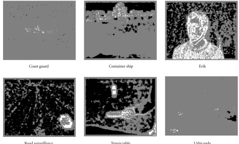
Coast guard Container ship Erik
Road surveillance Tennis table Urbicande
Figure2: Initial labelled sets.
standard deviations, or, equivalently, by the ratio of the two estimated parameters λ0 and λ1. Indeed, the Bhattacharya distance between the two distributions is equal to ln(λ0+ λ1)/2
λ0λ1. So we search for the closest frame which is suf-ficiently discriminated from the current one. Indeed, a value below the threshold means that the objects’ movement is small, and therefore it is difficult to detect the object. The threshold (Tλ) on the ratio of standard deviations is supplied
by the user, and thus is determined by the frame difference. In the case of a moving camera the frame difference is determined by the displaced frame difference of succes-sive frames. The camera movement must be computed for obtaining the displaced frame difference. We use a three-parameter model for describing the camera motion, com-posed of two translation parameters, (u, v), and a zoom pa-rameter,. The estimation of the three parameters is based on a frame matching technique with a robust criterion of least median of absolute displaced differences
min medianI(x, y, t)−I(x−u−x, y−v−y, t−1).
(3)
Only a fixed number of possible values for the set of mo-tion parameters (u, v,) is considered. Assuming convexity, we perform a series of refinements on the parameter space, a three-dimensional “divide-and-conquer” which yields the desired minimum within an acceptable accuracy after only four steps. In our implementation this requires the compu-tation of roughly one hundred values of the median of
ab-solute differences. For reasons of computational complexity the median is determined using the histogram of the absolute displaced frame differences.
3. CHANGE DETECTION USING FAST MARCHING ALGORITHM
3.1. Initial labelling
The labelling algorithm requires some initial correctly la-belled sets. For that we use statistical tests with high confi-dence for the initialisation of the label map. The percentage of points labelled by purely statistical tests depends on the ability to discriminate the two classes, which is related to the amount of relative object motion. For theCoast Guard se-quence (Figure 2), where it is difficult to distinguish the lit-tle boat, less than one percent of pixels are initialized. The background is shown in black, the foreground in white and unlabelled points in gray. For theEriksequence (Figure 2), for which the two probability density functions are shown in Figure 3, a large number of pixels are classified in the initial-ization stage.
The first test detects changed sites with high confidence. The false alarm probability is set to a small value, sayPF. The
threshold for labelling a pixel as “changed” is
T1= 1
λ0 ln 1
PF.
−025 −20 −15 −10 −5 0 5 10 15 20 25
Figure3: Mixture decomposition in Laplacian distributions for the inter-frame difference (Eriksequence).
Table1
Subsequently, a series of tests is used for finding unchanged sites with high confidence, that is, with a small probability of non-detection. For these tests a series of six windows of dimension (2w+ 1)2, w = 2, . . . ,7, is considered and the corresponding thresholds are preset as a function ofλ1. We denote by Bw the set of pixels labelled as unchanged
when testing the window indexed by w. We set them as follows: on the threshold γw, while λ1 is inversely proportional to the dispersion of d(x, y) under the “changed” hypothesis. As the evaluation of this probability is not straightforward, the numerical value of γw is empirically fixed. The
param-eter γ2 is chosen such that at least one pixel is labelled as “changed.” The other parameters (w=3, . . . ,7) are such that
γw =γw1 +γ2wvm, wherevmis proportional to the amount of
camera motion. In Table 1 we give the values used in our im-plementation.
Finally, the union of the above sets∪7
w=2Bw determines the initial set of “unchanged” pixels.
3.2. Label propagation
A multi-label fast marching level set algorithm is then ap-plied to all sets of points initially labelled. This algorithm is an extension of the well-known fast marching algorithm [17]. The contour of each region is propagated according
to a motion field, which depends on the label and on the absolute inter-frame difference. The label-dependent prop-agation speed is set according to the a posteriori probabil-ity principle. As the same principle will be used later for other level set propagations and for their respective veloc-ities, we shall present here the fundamental aspects of the definition of the propagation speed. The candidate label is ideally propagated with a speed in the interval [0,1], equal in magnitude to the a posteriori probability of the candi-date label at the considered point. We define the propagation speed at a site (x, y), for a candidate labelland for a data
Therefore the propagation speed depends on the likelihood ratios and on the a priori probabilities. The likelihood ratios can be evaluated according to assumptions on the data, and the a priori probabilities could be estimated, either globally or locally, or assumed all equal.
written as follows:
where the parameters λ0 andλ1 have been previously esti-mated. We distinguish the notation of the a priori probabili-ties defined here from those given in (2), because they should adapte to the conditions of propagation and to local situa-tions. Indeed, the above velocity definition is extended in or-der to include the neighbourhood of the consior-dered point
vl(x, y)=Pr
l(x, y)|d(x, y),kˆx, y,
x, y∈ᏺ(x, y), (9)
where the neighbourhood ᏺ(x, y) may depend on the la-bel, and may be defined on the current frame as well as on previous frames. Therefore, in this case the ratio of a priori probabilities is adapted to the local context, as in a Marko-vian model. A more detailed presentation of the approach for defining and estimating these probabilities follows.
From the statistical analysis of the data’s mixture distri-bution we have an estimation of the a priori probabilities of the two labels (P0, P1). This is an estimation and not a priori knowledge. However, the initially labelled points are not nec-essarily distributed according to the same probabilities, be-cause the initial detection depends on the amount of motion, which could be spatially and temporally variant. We define a parameterβmeasuring the divergence of the two probability distributions as follows:
pixels. The parameterβ0is fixed equal to 4 if the camera is not moving, and to 2 if the camera is moving. Thenβwill be the ratio of the a priori probabilities. In addition, forv1(x, y) the previous “change” map and local assignements are taken into account, and we define
Q0(x, y; 1) Q1(x, y; 1)=
eθ1−(α(x,y)+n1(x,y)−n0(x,y))ζ
β , (11)
where α(x, y) = η(x, y)−1, with η(x, y) the distance of the (interior) point from the border of the “changed” area on the previous pair of frames, andn1(x, y) (resp.,n0(x, y)) the number of pixels in neighbourhood already labelled as “changed” (resp., “unchanged”). The parameterζis adopted from the Markovian nature of the label process and it can be interpreted as a potential characterizing the labels of a pair of points. Finally, the exact propagation velocity for the “un-changed” label is
Absolute frame difference 0
Figure 4: The propagation speeds of the two labels; solid line: “changed” label, dashed line: “unchanged” label.
and for the “changed” label
v1(x, y) mentation the parameters are set as follows: θ0 = 4ζ and θ1=5ζ+ 4. In Figure 4, the two speeds are mapped as func-tions of the absolute inter-frame difference for typical pa-rameter values near the boundary.
We use the fast marching algorithm for advancing the contours towards the unlabelled space. Often in level set ap-proaches constraints on the boundary points are introduced in order to obtain a smooth and regularised contour and so that an automatic stopping criterion for the evolution is available. Our approach differs in that the propagation speed depends on competitive region properties, which both sta-bilises the contour and provides automatic stopping for the advancing contours. Only the smoothness of the boundary is not guaranteed. Therefore, the dependence of the propa-gation speed on the pixel properties alone, and not on con-tour curvature measures, is not a strong disadvantage here. The main advantage is the computational efficiency of the fast marching algorithm.
Hall monitor Mother and daughter Erik
Figure5: Change detection results.
The high-level description of the algorithm is as follows:
InitTValueMap() InitTrialLists()
while (ExistTrialPixels()) {
pxl=FindLeastTValue() MarkPixelAlive(pxl) UpdateLabelMap(pxl)
AddNeighborsToTrialLists(pxl) UpdateNeighborTValues(pxl) }
The algorithm is supplied with a label map partially filled with decisions. A map with pointers to linked lists of trial pixel candidacies is also maintained. These lists are initially empty except for sites neighbouring initial decisions. For those sites a trial pixel candidacy is added to the correspond-ing list for each different label of neighbourcorrespond-ing decisions and an initial arrival time is assigned. The arrival time for the initially labelled sites is set to zero, while for all others it is set to infinity. Apart from their participation in trial lists, all trial candidacies are maintained in a common priority queue, in order to facilitate the selection of the candidacy with the smallest arrival time.
While there are still unresolved trial candidacies, the trial candidacy with the smallest arrival time is selected and turned alive. If no other alive candidacy exists for this site, its label is copied to the final label map. For each neighbour of this site a trial candidacy of the same label is added, if it does not already possess one, to its corresponding trial list. Finally, all neighbouring trial pixels of the same label update their ar-rival times according to the stationary level set equation
∇T(x, y)= 1
v(x, y), (14)
wherev(x, y) corresponds to the propagation speed at point (x, y) of the evolving front, whileT(x, y) is a map of crossing times.
While it may seem that for a given site trial pixels can ex-ist for all different labels, in fact there can be at most four, since a trial candidacy is only introduced by a finalised deci-sion of a neighbouring pixel. In practice, trial pixels of
dif-ferent labels coexist only in region boundaries; therefore, the average number of label candidacies per pixel is at most two. Even in the worst case, it is evident that the time and space complexity of the algorithm is independent of the number of different labels. Experiments indicate a running time no more than twice that of the single contour fast marching al-gorithm.
4. MOVING OBJECT LOCALIZATION USING REGION GROWING ALGORITHM
4.1. Initialisation
The change detection stage could be used for initialisation of the moving object tracker. The objective now is to localize the boundary of the moving object. The ideal change area is the union of sites which are occupied by the object in two successive time instants
C(t, t+ 1)=O(t)∪O(t+ 1), (15)
whereO(t) is the set of points belonging to the moving object at timet. We also consider the change area
C(t−1, t)=O(t)∪O(t−1). (16)
It can easily be shown that the intersection of two successive change mapsC(t−1, t)∩C(t, t+ 1) is equal to
O(t)∪O(t+ 1)∩O(t−1). (17)
This means that the intersection of two successive change maps is a better initialisation for moving object localization than either one of them alone. In addition, sometimes
O(t+ 1)∩O(t−1)⊂O(t). (18)
If this is true, then
C(t, t+ 1)∩C(t, t−1)=O(t). (19)
Mother and daughter Erik
Figure6: Results on the uncertainty area.
Knowing also that there are some errors in change de-tection and that sometimes, under certain assumptions, the intersection of the two change maps gives the object approxi-mate location, we propose to initialize a region growing algo-rithm by this map, that is, the intersection of two successive change maps. This search will be performed in two stages: first, an area containing the object’s boundary is extracted, and second, the boundary is detected. The description of these stages follows.
4.2. Extraction of the uncertainty area
The objective now is to determine the area that contains the object’s boundary with extremely high confidence. Because of errors arising in the change detection stage, and also be-cause of the fact that the initial boundary is, in principle, placed outside the object, as shown in the previous subsec-tion, it is necessary to find an area large enough to contain the object’s boundary. This task is simplified if some knowl-edge about the background is available. In the absence of knowledge concerning the background, the initial boundary could be relaxed in both directions, inside and outside, with a constant speed, which may be different for the two direc-tions. Within this area then we search for the photometric boundary.
The objective is to place the inner border on the moving object and the outer border on the background. We empha-sise here thatinnermeans inside the object andoutermeans outside the object. Therefore, if an object contains holes the inner border corresponding to the hole includes the respec-tive outer border, in which case the inner border is expand-ing and the outer border is shrinkexpand-ing. In any case, the ob-ject contour is expected to be situated between them at every point and under this assumption it will be possible to deter-mine its location by the region-growing module described in Section 4.3. Therefore, the inner border should advance rapidly for points on the background and slowly for points on the object, whereas the opposite should be happen for the outer border.
For cases in which the background can be easily de-scribed, a level set approach extracts the zone of the ob-ject’s boundary. Suppose that the image intensity of the back-ground could be described by a Gaussian random variable
with meanµand varianceσ2. This model could be adapted to local measurements.
The propagation speeds will be also determined by the a posteriori probability principle. If, as assumed, the inten-sity on the background points is distributed according to the Gaussian distribution, the local average value of the intensity should also follow the Gaussian distribution with the same mean value and variance proportional toσ2. The likelihood test on the validity of this hypothesis is based on the nor-malised difference between the average and the mean value
¯
I−µ2
σ2 , (20)
where ¯Iis the average value of the intensity in a window of size 3×3 centered at the examined point. A low value means a good fit with the background. Therefore, the inner bor-der should advance more rapidly for low values of the above statistics, while the outer border should be decelerated for the same values.
On the other hand, it is almost certain that the border resulting from the previous stages is located on the back-ground. Thus the probability of being on the background is much higher than the probability of being on the object. For the outer border the speed is defined as
vb=
1 1 +cbe−4( ¯I−µ)2/σ2
, (21)
where it is considered that the variance of ¯Iis equal toσ2/8. According to (7) the constantcbis
cb=Pb Po
∆
σ√2π, (22)
wherePbandPoare the a priori probabilities of being on the
background or on the moving object, respectively. We have assumed that in the absence of knowledge the intensity of the object is uniformly distributed in an interval whose width is
∆(possibly equal to 255). As the initial contour is more likely located on the background,Pois given a smaller value than Pb(typicallyPb/Po=3). The outer border advances with the
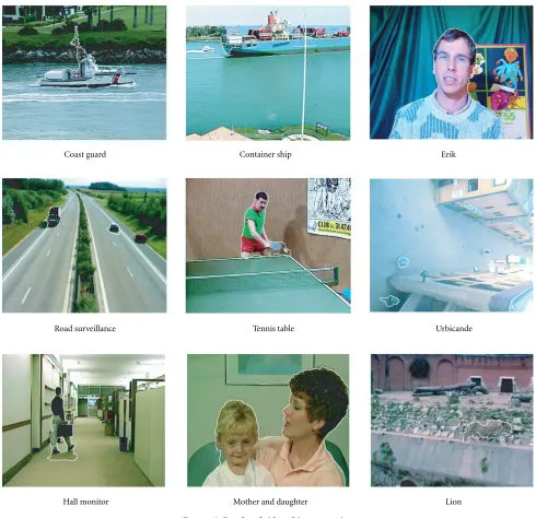
Coast guard Container ship Erik
Road surveillance Tennis table Urbicande
Hall monitor Mother and daughter Lion
Figure7: Results of video object extraction.
vo=1−vb, (23)
using the same local variance computation.
For cases in which the background is inhomogeneous, the uncertainty area is a fixed zone, where the two propaga-tion velocities are constant. They may be different in order to achieve the objective of placing the inner border on the mov-ing object and the outer border on the background. Result on theErikandMother and daughtersequences are shown in Figure 6.
The width of the uncertainty zone is determined by a threshold on the arrival times, which depends on the size of the detected objects and on the amount of motion and which provides the stopping criterion. At each point along the boundary, the distance from a corresponding “center”
point of the object is determined using a heuristic technique for fast computation. The uncertainty zone is a fixed per-centage of this radius modified in order to be adapted to the motion magnitude. However, motion is not estimated, and only a global motion indicator is extracted from the compar-ison of the consecutive changed areas. The motion indicator is equal to the ratio of the number of pixels with different la-bels on two consecutive “change” maps to the number of the detected object points.
4.3. Region growing-based object localization
la-belling technique, in which each step of the algorithm labels exactly one pixel, that with the lowest dissimilarity. In [22], the SRG algorithm was used for semi-automatic motion seg-mentation.
The segmentation result depends on the dissimilarity cri-terion, say δ(·,·). The colour features of both background and foreground are unknown in our case. In addition, local inhomogeneity is possible. For these reasons, we first deter-mine the connected components already labelled, with two possible labels: background and foreground. On the bound-ary of all connected components we place representative points, for which we compute the locally average colour vec-tor in theLabsystem. The dissimilarity of the candidate point from the already labelled regions during region growing pro-cess is determined using this feature as well as the Euclidean distance. After every pixel labelling, the corresponding fea-ture is updated. Therefore, we search for sequential spatial segmentation based on colour homogeneity, knowing that both background and foreground objects may be globally in-homogeneous, but presenting local colour similarities suffi-cient for their discrimination.
For the implementation of the SRG algorithm, a list that keeps its members (pixels) ordered according to the dissim-ilarity criterion is used, traditionally referred to as Sequen-tially Sorted List (SSL). With this data structure available, the complete SRG algorithm is as follows:
S1 Label the points of the initial sets.
S2 Insert all neighbours of the initial sets into the SSL. S3 Compute the average local colour vector for a
prede-termined subset of the boundary points of the initial sets.
S4 While the SSL is not empty:
S4.1 Remove the first point yfrom the SSL and la-bel it.
S4.2 Update the colour features of the representative to which the pointywas associated.
S4.3 Test the neighbours ofyand update the SSL: S4.3.1 Add neighbours of ywhich are neither
al-ready labelled nor alal-ready in the SSL, ac-cording to their value ofδ(·,·).
S4.3.2 Test for neighbours which are already in the SSL and now border on an additional set be-cause ofy’s classification. These are flagged as boundary points. Furthermore, if their
δ(·,·) is reduced, they are promoted accord-ingly in the SSL.
When SRG is completed, every pixel is assigned one of the two possible labels: foreground or background.
5. RESULTS AND CONCLUSION
We applied the above described algorithm to the entire COST data set. The results are given in our web page http://www.csd.uoc.gr/tziritas/cost.html
We obtained results ranging from good to very good, de-pending on the image sequence. Some segmented frames are shown in Figure 7. For comparison the spatial quality
mea-0 5 10 15 20 25 30 35 40 45 50
Figure8: Comparison based on the spatial quality measure for the Eriksequence.
Figure9: Comparison based on the spatial quality measure for the Hall monitorsequence.
sures [23] on the Erik (resp., Hall Monitor) sequence for the COST AM algorithm [14] and that of our algorithm are shown together in Figure 8 (resp., Figure 9). Our algorithm gives results of quality either similar to or better than the COST AM algorithm. The COST AM results, the reference segmented sequences, and the evaluation tool are taken from the web site http://www.tele.ucl.ac.be/EXCHANGE/
object localization can be further improved. The modeliza-tion of local colour and texture content could be possible, leading to a more adaptive region growing, or eventually a pixel labelling procedure.
ACKNOWLEDGMENTS
This work has been funded in part by the European IST PISTE (“Personalized Immersive Sports TV Experience”) and the Greek “MPEG-4 Authoring Tools” projects.
REFERENCES
[1] T. Sikora, “The MPEG-4 video standard verification model,” IEEE Trans. Circuits and Systems for Video Technology, vol. 7, no. 1, pp. 19–31, 1997.
[2] P. Salembier and F. Marques, “Region-based representations of image and video: segmentation tools for multimedia ser-vices,” IEEE Trans. Circuits and Systems for Video Technology, vol. 9, no. 8, pp. 1147–1169, 1999.
[3] T. Aach and A. Kaup, “Bayesian algorithms for adaptive change detection in image sequences using Markov random fields,”Signal Processing: Image Communication, vol. 7, no. 2, pp. 147–160, 1995.
[4] T. Aach, A. Kaup, and R. Mester, “Statistical model-based change detection in moving video,”Signal Processing, vol. 31, no. 2, pp. 165–180, 1993.
[5] M. Bischel, “Segmenting simply connected moving objects in a static scene,” IEEE Trans. on Pattern Analysis and Machine Intelligence, vol. 16, no. 11, pp. 1138–1142, 1994.
[6] K. Karmann, A. Brandt, and R. Gerl, “Moving object segmen-tation based on adaptive reference images,” inEuropean Signal Processing Conf., pp. 951–954, 1990.
[7] J.-M. Odobez and P. Bouthemy, “Robust multiresolution esti-mation of parametric motion models,”Journal of Visual Com-munication and Image Representation, vol. 6, no. 4, pp. 348– 365, 1995.
[8] Z. Sivan and D. Malah, “Change detection and texture analysis for image sequence coding,”Signal Processing: Image Commu-nication, vol. 6, no. 4, pp. 357–376, 1994.
[9] N. Paragios and G. Tziritas, “Adaptive detection and localiza-tion of moving objects in image sequences,”Signal Processing: Image Communication, vol. 14, no. 4, pp. 277–296, 1999. [10] M. Kass, A. Witkin, and D. Terzopoulos, “Snakes: active
con-tour models,”International Journal of Computer Vision, vol. 1, no. 4, pp. 321–331, 1988.
[11] A. Blake and M. Isard, Active Contours, Springer-Verlag, NY, USA, 1998.
[12] V. Caselles and B. Coll, “Snakes in movement,”SIAM Journal on Numerical Analysis, vol. 33, no. 6, pp. 2445–2456, 1996. [13] N. Paragios and R. Deriche, “Geodesic active contours and
level sets for the detection and tracking of moving objects,” IEEE Trans. on Pattern Analysis and Machine Intelligence, vol. 22, no. 3, pp. 266–280, 2000.
[14] A. Alatan, L. Onural, M. Wollborn, R. Mech, E. Tuncel, and T. Sikora, “Image sequence analysis for emerging interactive multimedia services—the European COST 211 framework,” IEEE Trans. Circuits and Systems for Video Technology, vol. 8, no. 7, pp. 802–813, 1998.
[15] M. Kim, J. G. Choi, D. Kim, et al., “A VOP generation tool: au-tomatic segmentation of moving objects on image sequences based on spatio-temporal information,” IEEE Trans. Circuits and Systems for Video Technology, vol. 9, no. 8, pp. 1216–1226, 1999.
[16] E. Sifakis, C. Garcia, and G. Tziritas, “Bayesian level sets for
image segmentation,” Journal of Visual Communication and Image Representation, vol. 13, no. 112, pp. 44–64, 2002. [17] J. A. Sethian, “Theory, algorithms, and applications of level
set methods for propagating interfaces,” Acta Numerica, vol. 5, pp. 309–395, 1996.
[18] E. Sifakis and G. Tziritas, “Fast marching to moving object location,” inProc.2nd Int. Conf. on Scale-Space Theories in Computer Vision, pp. 447–452, 1999.
[19] E. Sifakis and G. Tziritas, “Moving object localisation using a multi-label fast marching algorithm,”Signal Processing: Image Communication, vol. 16, no. 10, pp. 963–976, 2001.
[20] R. O. Duda and P. E. Hart, Pattern Classification and Scene Analysis, Wiley, NY, USA, 1973.
[21] R. Adams and L. Bischof, “Seeded region growing,” IEEE Trans. on Pattern Analysis and Machine Intelligence, vol. 16, no. 6, pp. 641–647, 1994.
[22] I. Grinias and G. Tziritas, “A semi-automatic seeded region growing algorithm for video object localization and tracking,” Signal Processing: Image Communication, vol. 16, no. 10, pp. 977–986, 2001.
[23] R. Mech and F. Marques, “Objective evaluation criteria for 2D-shape estimation results of moving objects,” in Proc. Workshop on Image Analysis for Multimedia Interactive Ser-vices, Tampere, Finland, May 2001.
Eftychis Sifakis was born in Heraklion, Crete on May 20, 1978. He received his B.S. in Computer Science (2000) from the Uni-versity of Crete. He received from Ericsson an award of Excellence in Telecommunica-tions for his B.S. thesis (2001). His research interests are in image analysis and pattern recognition.
Ilias Griniasreceived his B.S. (1997) and the M.S. (1999) in Com-puter Science from the University of Crete. His research interests are in image analysis and pattern recognition.
Georgios Tziritaswas born in Heraklion, Crete on January 7, 1954. He received the Diploma of Electrical Engineering (1977) from the Technical University of Athens, the “Diplome d’Etudes Approfondies” (DEA, 1978), the “Diplome de Docteur Inge-nieur” (1981), and the “Diplome de Doc-teur d’Etat” (1985) from the “Institut Poly-technique de Grenoble.” From 1982 he was a researcher of the “Centre National de