Evaluations on underdetermined blind source separation in adverse environments using time frequency masking

(1)

R E S E A R C H

Open Access

Evaluations on underdetermined blind source

separation in adverse environments using

time-frequency masking

Ingrid Jafari

1*

, Serajul Haque

1

, Roberto Togneri

1

and Sven Nordholm

2

Abstract

The successful implementation of speech processing systems in the real world depends on its ability to handle adverse acoustic conditions with undesirable factors such as room reverberation and background noise. In this study, an extension to the established multiple sensors degenerate unmixing estimation technique (MENUET) algorithm for blind source separation is proposed based on the fuzzyc-means clustering to yield improvements in separation ability for underdetermined situations using a nonlinear microphone array. However, rather than test the blind source separation ability solely on reverberant conditions, this paper extends this to include a variety of simulated and real-world noisy environments. Results reported encouraging separation ability and improved perceptual quality of the separated sources for such adverse conditions. Not only does this establish this proposed methodology as a credible improvement to the system, but also implies further applicability in areas such as noise suppression in adverse acoustic environments.

Keywords: Blind source separation; Fuzzy c-means clustering; Time-frequency masking; Reverberation; Background noise

1 Introduction

The ability of the human cognitive system to distinguish between multiple, simultaneously active sources of sound is a remarkable quality that is often taken for granted. This capability has been studied extensively within the speech processing community, and many an endeavor at imitation has been made. However, automatic speech processing systems are yet to perform at a level akin to human proficiency [1] and are thus frequently faced with the quintessential ‘cocktail party problem’: the inad-equacy in the processing of the target speaker/s when there are multiple speakers in the scene [2]. The imple-mentation of a suitable source separation algorithm can improve the performance of such systems, where source separation is the recovery of the original sources from a set of mixed observations. If no a prioriinformation of the original sources and/or mixing process is available, it is termed blind source separation (BSS). Rather than

*Correspondence: [email protected]

1School of Electrical, Electronic and Computer Engineering, The University of Western Australia, Crawley WA 6009, Australia

Full list of author information is available at the end of the article

rely on the availability of sucha prioriinformation, BSS methods often exploit an assumption on the constituent source signals and utilize spatial diversity obtained from the sensor observations. BSS has many important applica-tions in both the audio and biosignal disciplines, including medical imaging and communication systems.

In the last decade, the research field of BSS has evolved significantly to be an important technique in acoustic signal processing [3]. More specifically, the concept of time-frequency (TF) masking in the context of BSS has been of significance due to its applicability to all BSS scenarios, in particular the underdetermined case, where there exists more sources than sensors. In the TF masking approach to BSS, the assumption of sparseness between the speech sources is typically exploited as initiated in [4]. There exists several definitions for sparseness in the lit-erature; for example, [5] simply defines sparseness as to contain as ‘many zeros as possible’, whereas others offer a more quantifiable measure such as kurtosis [6]. Often, a sparse representation of speech mixtures can be acquired through the projection of the signals onto an appropri-ate basis, such as the Gabor or Fourier basis. In particular,

(2)

the W-disjoint orthogonality (W-DO) of speech signals was explored for the short-time Fourier transform (STFT) domain, where the sparseness implies that the STFT sup-ports of the signals are disjoint. This significant discovery motivated the degenerate unmixing estimation technique (DUET) [4]. The DUET proposed a demixing approach based on the formation of TF masks, where each mask would essentially correspond to the indicator function for the support of the source signal. The DUET algorithm suc-cessfully recovered the original source signals from stereo microphone observations using estimates of the relative attenuation and phase parameters.

The DUET algorithm consequently stimulated a plethora of demixing techniques. Among the first exten-sions to the DUET was the TF ratio of mixtures (TIFROM) algorithm which relaxed the sparseness assumption; how-ever its performance was limited to anechoic conditions with the observations idealized to be of the linear and instantaneous case [7]. Subsequent research extended the DUET to echoic conditions with the use of the estimation of signal parameters via rotational invariance technique (ESPRIT) method to form the DUET-ESPRIT algorithm [8,9]. However, this was restricted to a linear microphone arrangement and was thus subjected to front-back con-fusions primarily due to the natural constraint in spatial diversity from the microphone observations.

A different avenue of research as in [10] composed a two-stage algorithm which combined the sparseness principle presented in DUET with the established inde-pendent component analysis (ICA) algorithm to yield the sparseness and ICA (SPICA) algorithm. This approach exploited the sparseness of the signals to estimate and remove the active speech source at a particular TF point, and ICA was then applied to the remaining mixtures. Nat-urally, a restraint upon the number of sources present at any TF point relative to the number of sensors was inevitable due to the ICA stage. Furthermore, the algo-rithm was only investigated for the stereo case.

The authors of the SPICA expanded their research to nonlinear microphone arrays in [11-13] with the intro-duction of the clustering of normalized observation vec-tors. Whilst remaining similar in spirit to the DUET, the research was inclusive of non-ideal conditions such as room reverberation, and allowed more than two sen-sors in an arbitrary arrangement. This eventually culmi-nated in the development of the multiple sensors degen-erate unmixing estimation technique, termed MENUET [14,15]. Additionally, the mask estimation in MENUET was automated through the application of the k-means clustering technique. Another algorithm which proposes the use of a clustering approach for the mask estima-tion is presented in [16]: this study is based upon the concept of Hermitian angles between the reference vec-tor and observation vecvec-tors, in the complex vecvec-tor space.

However, evaluations were restricted to a linear micro-phone array.

Advancements in the TF masking approaches to BSS beyond MENUET involve additional stages and complex-ities. Of particular mention is the approach in [17] which resulted in superior BSS performance in underdetermined reverberant conditions. The algorithm employed a two-stage approach: firstly, observation vectors are clustered in a frequency bin-wise manner, and secondly, the sepa-rated frequency bin components classified as originating from the same source are grouped together. The bene-fit of this approach is that due to the bin-wise clustering, it is robust against higher room reverberations in com-parison to previous techniques such as MENUET, as well as possessing an inherent immunity to the spatial alias-ing problem in the measurement of the time differences of arrival/direction of arrivals [17]. However, despite the reported improvements in BSS performance, additional complexity was introduced due to the extra stage for the alignment of the frequency bin-wise permuted clustering results. Therefore, the MENUET has the advantage over the state-of-the-art study in [17] in that the fullband clus-tering for mask estimation eliminates the requirement for the additional stage of frequency bin-wise alignment.

However, the simplicity encapsulated in the MENUET inevitably presents its own limitations. Most significantly, thek-means clustering utilized for mask estimation is not highly robust in the presence of outliers or interference in the data. This often leads to non-optimal localization and partitioning results, particularly for reverberant mix-tures [18,19]. Furthermore, binary masking schemes have been shown to impede upon the separation quality due to musical noise distortions, and it was suggested that fuzzy masking approaches bear the potential to signifi-cantly reduce the musical noise at the output [12]. This may be attributed to the fact that when a hard partitioning approach is implemented, abrupt changes will exist in the recovered source estimate which consequently introduce artifacts in the time domain.

The suitability of fuzzyc-means (FCM) clustering for TF mask estimation in the BSS framework has been explored in [20,21]. In this approach, the fuzzy partitioning in the c-means was suggested to be preferable to hard clustering due to the inherent ambiguity surrounding the member-ship of TF cells to a cluster, where examples of contribut-ing factors to ambiguity include the effects of reverber-ation and environmental (background) noise. However, the investigations to date which employ the FCM, as with many others in the literature, have been restricted to a linear and overdetermined microphone arrangement.

(3)

individual component densities of the GMM may model some underlying set of hidden parameters in a mixture of sources. Due to the reported success of BSS methods that employ such Gaussian models, this clustering paradigm may be considered as a standard algorithm for comparison of mask estimation ability in the TF BSS framework, and is therefore investigated and regarded as a comparative model in this study.

However, each of the TF mask estimation approaches to BSS discussed above are limited in their evaluations with respect to the fact that diverse sources of interference are not considered. Potential contributors to interference in BSS scenarios include not only room reverberation, but also environmental background noise, or noise originating from non-ideal recording sensors. In fact, almost all real-world applications of BSS have the inconvenient aspect of noise at the recording sensors [25], and the influence of such noise has been described as a very difficult and continually open problem in the BSS framework [26].

In general, the focus of BSS algorithms is not directed towards the suppression of environmental noise. How-ever, for a system to achieve optimal performance, the impact of such noise must be addressed. Numerous stud-ies in the literature have been proposed for the problem of additive sensor noise: Li et al. [27] present a two-stage denoising/separation algorithm; Cichocki et al. [25] implement a FIR filter at each channel to reduce the effects of additive noise; and Shi et al. [28] suggest a pre-processing whitening procedure for enhancement. The study in [29] considers a variety of common sources of background noise in the separation algorithm, and modifies numerous pre- and post-processing algorithms in order to account for the characteristics of the back-ground noise. Whilst noise reduction has been achieved with denoising techniques implemented as a pre- or post-processing step, the performance was proven to degrade significantly at lower signal-to-noise ratios [30].

Within the TF BSS framework, the authors of [22] include the possibility of background noise in the observation error for their BSS model; however, the experimental simulations were only conducted for ane-choic/reverberant conditions, without any clear distinc-tion between environmental noise and reverberadistinc-tion in the observation error.

Motivated by such various shortcomings, this work presents an extension to the MENUET algorithm through the use of an alternative clustering scheme for mask estimation, and provides comprehensive evaluations in adverse acoustic conditions. Firstly, this study proposes that the substitution of the TF clustering stage with a fuzzy clustering approach as explored in [20,21] will improve the separation performance in the same condi-tions as presented in [14,15]. Secondly, it is hypothesized that this combination is sufficiently robust to withstand

the degrading effects of reverberation and environmental noise, and evaluations of all the methods under the chal-lenging conditions of reverberation and environmental background noise are presented. For all investigations in the study, comparisons are provided with both the origi-nal MENUETk-means and the standard soft GMM-based clustering algorithm for mask estimation.

The remainder of this paper is organized as follows: section 2 provides an overview of the proposed BSS scheme and explains the primary signal processing stages. Section 3 describes each of the three clustering schemes in greater detail. Section 4 explains the experimental eval-uation and presents a discussion on the achieved results. The section also includes the existing limitations with the system and offers some potential avenues for future work. Section 5 concludes the paper with a brief summary.

2 System overview

2.1 Problem statement

Consider a microphone array ofM identical sensors in a reverberant enclosure whereN sources are present. A convolutive mixing model is assumed, whereby the obser-vation at the mth sensor, xm(t), can be modeled as a

summation of the individual contributions by the nth active source,sn(t).

When allN sources are active, the observation at the mth sensor can be expressed via the convolutive mixing model as

xm(t)= N

n=1

p

hmn(p)sn(t−p)+nm(t), (1)

wherehmn(p)p= 0,. . .,P−1 denote the coefficients of

the room impulse response between thenth source to the mth sensor,nm(t)denotes any additive noise received at

themth sensor andtindicates time.

The goal of any BSS system is to therefore recover the N sources,sˆ1,. . .,ˆsN, each of which corresponds to the

original source signalss1,. . .,sN, respectively. Ideally, the

separation is performed without any information about sn(t)andhmn(p).

2.2 STFT analysis

The time-domain sensor observations are converted into their corresponding frequency domain time-series Xm(k,l)via the STFT as

Xm(k,l)= L/2−1

τ=−L/2

win(τ )xm(τ+kτ0)e−jlω0τ, m=1,. . .,M,

(2)

(4)

are the TF grid resolution parameters. The analysis win-dow is typically chosen such that sufficient information is retained within whilst simultaneously reducing signal dis-continuities at the edges. A suitable window is the Hann window:

win(τ )=0.5−0.5cos(2π τ

L ), τ =0,. . .,L−1, (3)

whereLdenotes the frame size.

It is assumed that the length ofLis sufficient such that the main portion of the impulse responseshmnis covered.

Therefore, the convolutive BSS problem may be approx-imated as an instantaneous mixture model [31] in the STFT domain

where (k,l) represent the time and frequency index, respectively and Hmn(l) is the room impulse response

between source n and sensor m. Sn(k,l), Xm(k,l) and Nm(k,l)are the STFT of thenth source,mth observation

and additive noise at themth sensor, respectively.

The assumption of sparseness between the source sig-nals implies that at each TF cell, at most one source is dominant [4]. Therefore, (4) can be expressed as

Xm(k,l)≈

whereδ_n(k,l)is the Dirac-delta function defined as

δn(k,l)=

1 whenSn(k,l)is active at(k,l),

0 otherwise. (6)

Whilst this sparseness assumption holds true for ane-choic mixtures, as the reverberation and/or environ-mental noise in the acoustic scene increases it becomes increasingly unreliable due to the effects of multipath audio propagation and multiple reflections [4,21].

2.3 Feature extraction

In this work, the TF mask estimation is realized through the estimation of the TF points where a signal is assumed dominant. To estimate such TF points, a spatial feature vector is calculated from the STFT representations of the Mobservations. Previous researches [14,15] have identi-fied level ratios and phase differences between the obser-vations as appropriate features, as such features retain information on the magnitude and the argument of the TF points. Further discussion is presented in section 4.3.1.

The feature vectorθ(k,l) = θL(k,l),θP(k,l)T per TF

where f is the frequency at thelth frequency bin index, cis the propagation velocity of sound,dmax is the

maxi-mum distance between any two sensors in the array and Jis the index of the (arbitrarily selected) reference sensor. The weighting parameters A(k,l) and α ensure appro-priate amplitude and phase normalization of the features respectively. It is widely known that in the presence of reverberation, a greater accuracy in phase ratio measure-ments can be achieved with higher spatial resolution; however, it should be noted that the value ofdmaxis upper

bounded by the spatial aliasing theorem [14,17,21]. If the exact value of the maximum sensor spacing is not known, a positive constant may be used in its place [14]. This elim-inates the need for the system to know the precise spacing between sensors.

The frequency normalization in (8) ensures frequency independence of the phase ratios in order to prevent the frequency permutation problem in the later stages of clus-tering. It is possible to cluster without such frequency independence by implementing a bin-wise clustering as in [17,32]. However, the utilization of all the frequency bins avoids the frequency permutation problem and also permits data observations of short length [14].

2.4 Mask estimation and separation

In this work, source separation is effected through the estimation and application of TF masks, which are esti-mated in the clustering stage. For thek-means algorithm, a binary mask for the nth source is simply estimated as [14]

Mn(k,l)=

1 forθ(k,l)∈Cn,

0 otherwise. (9)

whereCndenotes the set of TF points classified as

belong-ing to thenth cluster.

(5)

the degree of membership of each TF point in the feature space to each of theNclusters. These membership values, denoted byun(k,l), are then interpreted as a collection of NTF masks:

Mn(k,l)=un(k,l). (10)

For the GMM clustering approach, the mask is set to the posterior probabilities of the dominant Gaussian components (cf. section 3.2) [22,23]. This equates to

Mn(k,l)=p(θ(k,l)|μk,k), (11)

whereμp,pdenotes the mean and covariance matrix of

thepth Gaussian component of the mixture model. The spatial image estimate of thenth signal received at themth sensor is then obtained through the application of maskMnto themth observation as [17]

ˆ

Smn(k,l)=Mn(k,l)Xm(k,l), n=1,. . .,N. (12)

2.5 Source resynthesis

Finally, the estimated source images are reconstructed in the time-domain to obtain the estimates ˆsmn(t). This is

realized through the overlap-and-add method [34] onto ˆ

Smn(k,l). The reconstructed estimate is

ˆ smn(t)=

1 Cwin

L/τ0−1

k=0 ˆ

sk_mn+k(t), (13)

whereCwin = 0.5/τ0L is a Hann window function

con-stant, and individual frequency components of the recov-ered signal are acquired through an inverse STFT

ˆ sk_mn(t)=

L−1

l=0 ˆ

Smn(k,l)ejlω0(t−kτ0), (14)

if(kτ0≤t≤kτ +L−1), and zero otherwise.

3 Clustering approaches

This section presents the details of the three clustering techniques employed in this study. The first two, the hard k-means and the Gaussian mixture model, have previ-ously been used in other TF-based clustering BSS sys-tems [14,24], whilst the fuzzy c-means is the proposed mask estimation technique. All three techniques belong to the family of center-based clustering, and each have their own objective functions. The common goal of all is the classification of the set of feature vectors,(k,l) = {θ(k,l)|θ(k,l) ∈ R2(M−1)_,_(k_,_l) _∈ _}_{, where} _{= {}_(k_,_l) _:

0 ≤ k ≤ K−1, 0 ≤ l ≤ L−1}denotes the set of TF points in the STFT plane, intoNclusters. In the instance where the clusters are distinct, as with the hardk-means, each data point may only belong to one cluster. How-ever, for the soft clustering techniques, each data element may belong to multiple clusters with a certain probability (membership).

3.1 Hardk-means clustering

Previous mask estimation methods as in [13-16] employ binary clustering techniques such as the hard k-means (HKM). The HKM algorithm was initially introduced in studies published by MacQueen [35]. In this approach, the set of feature vectors(k,l) is clustered intoN distinct cluster sets{C} =C1,. . .,CN. Each set from{C}contains

the feature vectors assigned to thenth cluster, and has an associated set of prototype vectors,vn, which denotes the nth cluster center.

Clustering of the data is achieved through the minimiza-tion of the objective funcminimiza-tion

JHKM= N

n=1

θ(k,l)∈Cn

Dn(k,l), (15)

whereDn(k,l)= θ(k,l)−vn2is the squared Euclidean

distance between the feature vector θ(k,l) and the nth cluster center.

Conditional on a set of initial centroids, this minimiza-tion is iteratively realized by the following alternating equations

C_n∗= {θ(k,l)|n=argmin

n

Dn(k,l)}, ∀n,k,l, (16)

vn∗←E{θ(k,l)}θ(k,l)∈Cn, ∀n, (17)

until convergence is met, whereE{.}θ(k,l)∈Cn denotes the

mean operator for the TF points within the cluster setCn,

and the (*) operator denotes the optimal value (at conver-gence). Due to the algorithm’s sensitivity to initialization of the cluster centers it is recommended to either design initial centroids using an assumption on the sensor and source geometry as in [14,15], or to utilize the best out-come of a predetermined number of independent runs.

Summary: HKM clustering algorithm

Input:θ(k,l),N

Output:V∗_HKM,{C}∗_HKM

1. Initialise set of centroidsV(0)= {vn|∀n∈ {1,. . .,N}}

randomly

Repeatforj=1, 2,. . .,

2. Compute distancesD(j)_with_V(j−1)

3. Update cluster sets{C}(j)using (16)

4. Update centroidsV(j)with{C}(j)using (17)

5. Until predetermined number of runsJ∗reached

Return V∗_HKM←V(J∗)and{C}∗_HKM← {C}(J∗)

3.2 Gaussian mixture model clustering

(6)

and it is therefore included in this study for compara-tive purposes. It is also included in order to compare the effects of soft masking on the separation system, by providing the FCM with a fair comparison.

In the GMM-based clustering, each observationθ(k,l) can be modeled as a weighted sum of P component Gaussian densities (clusters). Unlike the HKM and FCM described above, where the number of clusters is equal to the number of sources, the GMM-based clustering meth-ods have the additional complexity in that the best fitting for the data set to a mixture model may not necessitate thatPis equivalent to the number of sources [14].

Thepth component of the mixture model is assumed to follow a Gaussian distribution with a characteristic mean and covariance,μp andp, respectively. The probability

density function of an observationθ(k,l), denoted byθfor simplicity from here onward, is represented mathemati-cally as:

where (μ,) contains the mean and covariance matri-ces for allPclusters, andwpdenotes the mixture weight

(probability) of thepth distribution. Thispth component density is represented by

butions are estimated in such a manner as to maximize the likelihood of the mixture model; this estimation is most commonly iteratively calculated using the Expectation-Maximization (EM) algorithm [22]. The data is then clustered around the maximum likelihood parameters as determined from the EM algorithm by the final estimates of thea posterioriprobabilities at convergence.

Conditional on an initial partitioning, that is the initial cluster sets {C1,. . .,CP} are known, the parameters sets

The cluster sets are then found by assigning poste-rior probabilities to the mixture components. The use of GMM clustering within this particular BSS framework results in the number of components not equal to the number of sources (see section 4.1); therefore, the domi-nantNcomponents of theP, as determined by the mixture weights, are selected to represent theNsources. The pos-terior probabilities of the dominant Gaussians, denoted p(θ|μ_p,_p), are then utilized as the TF mask to repre-sent the corresponding source (analogous to the work in [14,17]).

3.3 Fuzzyc-means clustering

Whilst the HKM performed satisfactorily in the context of MENUET for BSS, the work presented in [21] and [36] demonstrated that the use of a fuzzy clustering algorithm improves the accuracy of mask estimation. The origins of the FCM are credited to the work presented in [33], and as with the HKM method, the feature set is clustered into N clusters, where each cluster center is represented by a centroidvn. However, each cluster also has an associated partition matrixU= {un(k,l)∈R|n∈(1,. . .,N),(k,l)∈ )}which specifies the probabilityun(k,l)to which a

fea-ture vectorθ(k,l)belongs to thenth cluster at the TF point (k,l).

Clustering is achieved by the minimization of the cost function

whereun(k,l)is subject to the constraint N

n=1

un(k,l)= 1

and withDn(k,l)defined as in section 3.1. The

fuzzifica-tion parameterq > 1 controls the membership softness in the cost function and therefore controls the fuzzi-ness of the generated TF masks. Section 4.1 describes the selection of an appropriate value for the fuzzification parameter in this BSS context.

(7)

u∗_n(k,l)= ⎡ ⎣N

j=1

Dn(k,l)

Dj(k,l)

1

q−1 ⎤ ⎦

−1

, ∀n,k,l, (24)

where (*) denotes the optimal value, until a suitable ter-mination criterion is satisfied. Typically, convergence is defined as when the difference between successive parti-tion matrices is less than some predetermined threshold, [33]. However, as is also the case with thek-means, it is known that the alternating optimization scheme pre-sented may converge to a local, as opposed to global, optimum; thus, it is suggested to independently imple-ment the algorithm several times prior to selecting the most fitting result [21].

Summary: FCM clustering algorithm

Input:θ(k,l),N

Output:U∗_FCM,V∗_FCM

1. Initialise partitionU(0)randomly

Repeatforj=1, 2,. . .,

2. Update centroidsV(j)withU(j−1)using (23)

3. Compute distancesD(j)_with_V(j)

4. Update partition matrixU(j)withD(j)_{using (24)}

5. Until||U(j)−U(j−1)||<

Return U∗_FCM←U(j)andV∗_FCM←V(j)

4 Experimental evaluations

4.1 Experimental setup

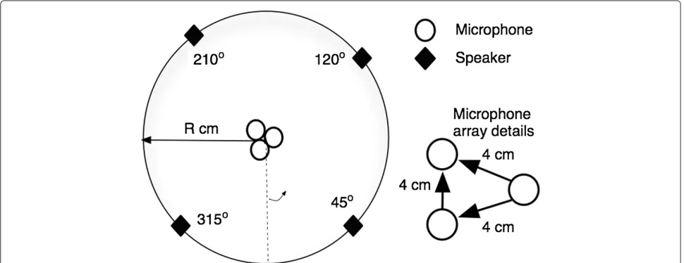
The experimental setup was designed to replicate that of the studies in [14,15] for comparative purposes. Figure 1 depicts the speaker and sensor arrangement, and Table 1 details the experimental conditions. The wall reflections

Table 1 The parameters used in experimental evaluations

Parameter Value

Number of sensors M= 3

Number of sources N= 4

R 50 cm

Signal length 6 s

Reverberation time 0 ms, 128 ms, 300 ms

Environment SNR −10 dB to 30 dB

Sampling rate 8 kHz

STFT window Hann

STFT frame size 64 ms

STFT frame overlap 50 %

of the enclosure and room impulse responses between each source and sensor were simulated using the image model method for small-room acoustics [38]. The room reverberation was quantified in the measure RT60, where

RT60 is defined as the time required for reflections of a

direct sound to decay by 60 dB below the level of the direct sound.

Several types of background noise can be described by a diffuse sound field and modeled by an infinite num-ber of statistically independent point sources on a sphere [29]. In this model, the intensities of the incident sound are uniformly distributed over all possible directions, and can be modeled as additive noise at the sensors, as in (1) [29]. In this study, 30 individual and independent point sources were situated uniformly from the center of the microphone array at a distance of 1.5 m. In an effort to gain adversity in the evaluations, three types of environmental noise were considered: white noise, babble noise and factory noise. All noise samples are available in

(8)

the NOISEX-92 database [39]. The simulated background noise was scaled according to the signal-to-noise ratio (SNR) definition as in [40], which uses the standardized method given by the International Telecommunications Union to objectively measure the active speech level and calibrate the interfering noise signal appropriately [41]. It should be noted that in real-world environments, noise is never exactly isotropic; therefore, these evaluations must be considered with caution.

The four target speech sources, the genders of which were randomly generated, were realized with phonetically-rich utterances from the TIMIT database [42], and the target-to-masker ratio between all of the sources was set to 0 dB. A representative number of mixtures for evaluative purposes was constructed. To avoid any spatial aliasing, the sensors were placed at a maximum distance of 4 cm apart.

Section 3.3 explains the role of the fuzzification param-eter q in the FCM clustering. Past research [21] has identified a value of q in the range of q ∈ (1, 1.5] to result in performance akin to hard clustering. Further-more, it was empirically determined that for reverberant speech mixtures, a value ofq = 2 is an optimal value in order to achieve a balance between high separation per-formance with minimal artifacts [21]. This is consistent with other studies which also report an optimal value at 2 for the fuzzy exponent [43,44]. Therefore, in this work, the fuzzificationqis set to 2.

As mentioned in sections 3.1 and 3.3, it is widely rec-ognized that the performance of the clustering algorithms is largely dependent on the initilization of the algorithm [19,45]. If the initial partitions are not estimated with suf-ficient precision, there is a high possiblity of finding a local, as opposed to global, optimum. It has been rec-ommended [19] to run the algorithms multiple times to reduce the degrading effects of its sensitivity; the effec-tiveness of this style of initialization was also described in [46]. In an effort to save computational expense, it was desired to determine the smallest number of indepen-dent, single-iteration runs for initialization which would result in the best solution. Previous experiments as in [21] had implemented the best of 50 runs; however, it was empirically confirmed that there was little differ-ence in performance between 25 and 50 runs. Therefore, it can be assumed that satisfactory clustering initializa-tion can result when the best soluinitializa-tion of 25 indepen-dent, randomly initialized single-iteration executions are selected for initilization. The ‘best’ solution was defined as the execution which resulted in the lowest cost function output of the independent runs (i.e. the smallest error).

Similar to the HKM and FCM algorithms, the GMM clustering approach also requires a suitable initialization. As recommended in [47], an initialization based on the Forgy method [48] was implemented, where the data set

was randomly partitioned into K non-overlapping sets with uniform mixing proportions. The initial covariance matrices for all components were diagonal. However, the GMM clustering approach is also highly sensitive to the selection of an appropriate number of components in the model. It was observed in the experiments that an increase in the number of mixture components generally resulted in improved separation performance; however, the selec-tion of an optimal number of Gaussians was not simple and required a considerable amount of experimentation in order to reach the optimal number. For this partic-ular application of the GMM clustering in the desired source/sensor configuration, it was empirically deter-mined asK =12. This is in accordance to previous studies using GMM for BSS such as in [14], where the determina-tion of the optimal number of clusters was at a consider-able computational expense. As mentioned in section 3.2, since the number of components are not equal to the number of sources, the dominantNcomponents (as indi-cated by the mixture weights) were used to estimate the TF separation masks. The TF masks were derived from the posterior probabilities of the dominant components.

4.2 Evaluation measures

In order to provide a comprehensive evaluation of the separation algorithms presented in this study, a range of performance metrics have been included. These include the widely used BSS_EVAL toolkit [49], the Perceptual Evaluation of Speech Quality measure (PESQ) [50] and the objective measures in the Perceptual Evaluation methods for Audio Source Separation (PEASS) toolkit [51].

4.2.1 BSS EVAL performance metrics

The first set of performance metrics was obtained from the publicly available MATLAB toolkit BSS_EVAL [49]. This set of metrics is applicable to all source separation approaches, and no prior information of the separation algorithm is required. However, the original toolkit does not account for environmental noise in the metrics. To account for this, an author of the BSS_EVAL was con-sulted in order to modify the toolkit to consider the addition of two extra metrics: the SNR and signal-to-interference-plus-noise ratio (SINR).

Using a least-squares projection, theBSS_EVALtoolkit assumes the decomposition of the estimated spatial image ˆ

smn(t)as

ˆ

smn(t)=simgmn(t)+espatmn(t)+einterfmn (t)+eartifmn(t)+enoisemn (t), (25)

wheremis the observation index,simgmn(t)is the true source

image andespatmn(t), einterfmn (t), eartifmn(t)andenoisemn (t)are

(9)

From this decomposition, the SIR was computed as [52]

SIRn=10log10 M m=1 t(s

img

mn(t)+espatmn(t))2 M

m=1 teinterfmn (t)2

(26)

to provide an estimate of the relative amount of interfer-ence in the target source estimate.

The SINR was computed as

SINRn=10log10 M m=1 t(s

img

m=1 t(enoisemn (t)+einterfmn (t))2

(27)

to reflect the amount of noise and interference in the recovered signal estimate.

The global SNR for thenth source was calculated as

SNRn=10log10 M m=1 t(s

img

mn(t)+espatmn(t)+einterfmn (t))2 M

m=1 tenoisemn (t)2

(28)

which provides a measure of the amount of noise at the recovered signal, independent of the interference. For all ratios, a higher value indicates better separation performance.

4.2.2 PESQ

The PESQ measure was originally designed to provide a subjective judgement of the speech quality of the recovered source signal. Despite its initial intention for telecommunication applications, it has since been shown to be an effective predictor for the quality of the speech isolated from the observation mixtures by the separation algorithm [53], as well as for ASR performance on the separated speech signals [54].

The PESQ score is computed by a comparison of the original (unmixed, anechoic) speech source signal to the recovered signal estimate. Both signals are time-aligned and passed through an auditory transform to achieve a psychoacoustically motivated representation [55]. The differences between the signals in this representation are measured and used to provide an estimate of the distor-tion in the signal estimate. The final measure of PESQ is reported to correlate well with subjective listening scores [53].

The PESQ score can take on a range from 0.5 to 4.5, where 4.5 represents the case when the signal estimate is equivalent to the original (clean) source. A higher score suggests better speech quality.

4.2.3 PEASS

The PEASS toolkit was created to provide a set of objec-tive scores to predict the perceptual quality of estimated sources. This is complementary to the energy-based ratios in theBSS_EVAL (cf. section 4.2.1), and the PEASS has since been implemented as a standard for performance

evaluation in international speech challenges such as the signal separation evaluation campaign (SiSEC) [52,56].

In this toolkit, the estimated signals are decomposed via a complex, auditory-motivated algorithm as [51]

ˆ

sn(t)−sn(t)=etarget(t)+einterf(t)+eartif(t), (29)

where sn(t) is the original (clean) target signal, and the

termsetarget(t),einterf(t)andeartif(t)denote the target

dis-tortion component, interference component and artifacts component, respectively. The salience of these error com-ponents is then measured using the perceptual similarity measure provided in the PEMO-Q auditory model [57]; the reader is referred to [51] for a detailed discussion.

The PEASS toolkit computes four auditory-motivated quality scores; however, the overall perceptual score (OPS) is considered as a global measure for the separation ability as it indicates the similarity between the recovered signal estimate and the original signal, and it is said to have a high coherence with the subjective perceptual evaluation. Therefore, in this study, the OPS is included as an addi-tional performance metric for the perceptual quality of the speech. The OPS is expressed from 0 to 100, where 100 denotes the best perceptual match.

4.3 Results

4.3.1 Initial evaluations of MENUET with FCM

Prior to evaluating the effectiveness of the FCM cluster-ing for mask estimation in the MENUET framework, the FCM was evaluated in a simple stereo setup for a variety of feature sets in order to test its feasibility in this context. In [14,15], a comprehensive review of suitable location cues was presented and their effectiveness at separation was evaluated using the HKM clustering for mask estimation.

The experimental setup for these set of evaluations was such as to replicate the original work in [14] to as close a degree as possible. In an enclosure of dimen-sions 4.55 m×3.55 m×2.5 m with a room reverberation parameter RT60constant at 128 ms, two omnidirectional

microphones were placed at a distance of 4 cm apart at an elevation of 1.2 m. Three speech sources, with a target-to-masker ratio of 0 dB, were situated at 30°, 70° and 135° at a distance of 50 cm from the array, and also at an elevation of 1.2 m. The speech sources were randomly chosen from both genders of the TIMIT database in order to emulate the investigations in [14,15] which utilized English utter-ances. The source separation performance was evaluated with respect to the improvement in SIR and the results are depicted in Table 2.

(10)

Table 2 The hardk-means and fuzzyc-means are

The reverberation was constant at RT60= 128 ms. The highest achieved ratios are emphasized in italics.

SIR gain that the FCM clustering is more robust than the original HKM for all but one feature set, and thus hints at the possibility of the FCM yielding similar results for related TF BSS approaches. Not only does this confirm the suitability of the FCM in the proposed BSS frame-work, it also demonstrates the robustness of the FCM against several types of spatial features. The results of this investigation provide further motivation to extend the soft TF masking scheme to other sensor arrangements and adverse acoustic conditions.

However, in the original evaluations in [14] the authors also compare the performance of the HKM for the same stereo, three speaker setup against the more robust GMM fitting clustering approach. The results of this demon-strated improvements in SIR gain in comparison to the HKM, although this was at the burden of significantly greater computational expense. Furthermore, the selec-tion of the number of Gaussian components proved to require a lot of trial and error (cf. section 4.1). In order to offer a fair comparison of the FCM against other clus-tering techniques, the GMM fitting method was then implemented in further BSS evaluations as stated in the following sections.

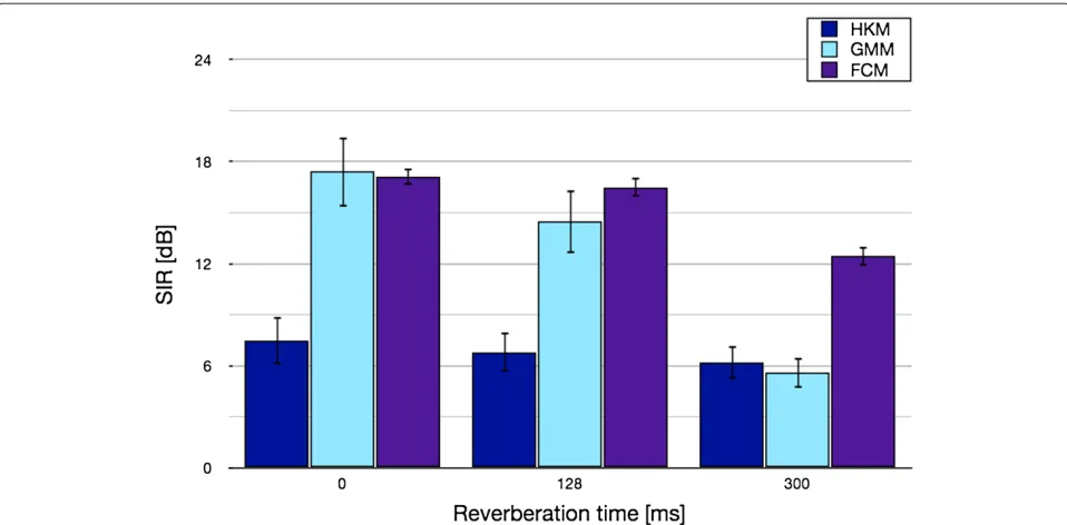
4.3.2 Separation in reverberant conditions

The study was extended to the underdetermined case of three sensors and four sources in a nonlinear configura-tion as in Figure 1 [14,15]. The average improvement in SIR measured across all separated sources for all evalu-ations is depicted in Figure 2, where the average input SIR was measured at−4.20 dB (consistent with the stud-ies in [14,15]). It is immediately evident that the two soft

masking techniques, GMM and FCM, improve the sep-aration quality by a considerable amount. For example, for the anechoic scenario, the GMM and FCM clustering techniques perform equivalently, leading the HKM mask estimation by almost 10 dB. However, as the reverberation is increased to a mild 128 ms, a slight performance gap between the two soft masking techniques surfaces with the FCM leading by approximately 2 dB. This gap is heightened as the reverberation is increased again, with the performance gap considerably larger at almost 7 dB. Interestingly, at this higher reverberation time, the GMM performs even below the HKM.

A smaller standard deviation is also observed in Figure 2 when FCM clustering is used. For example, when the reverberation is RT60 = 128 ms, the SIR performance

using GMM clustering is comparable to that of FCM clus-tering. However, the standard deviation is more than twice that of the FCM clustering, and this suggests that the FCM delivers more consistent and reliable separation of the sources.

To evaluate the statistical significance of the evaluations, the Student’sttest was conducted for the three methods, where two tests were conducted per RT60 value: one to

compare the statistical significance of the FCM against the HKM, and one to compare the FCM against the GMM. A two-tailed distribution was assumed for each test, with unequal variances between the data. For the FCM against the HKM, apvalue ofp << 0.001 was reported for all reverberation times. For the FCM against the GMM, for a reverberation time of RT60 =0 ms, apvalue of less than

0.1 (p = 0.094) was measured. However, for the remain-ing reverberation times, a p value of p << 0.001 was recorded. This demonstrates that the performance of the proposed FCM mask estimation is largely unlikely to be due to chance. Therefore, the performance of the FCM clustering indicates a superior mask estimation technique for source separation in a reverberant enclosure.

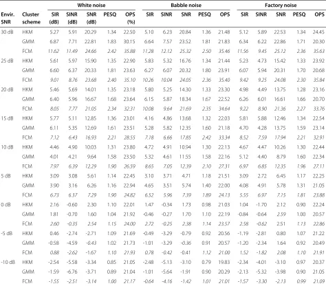
4.3.3 Separation in reverberant conditions with spatially diffuse environmental noise

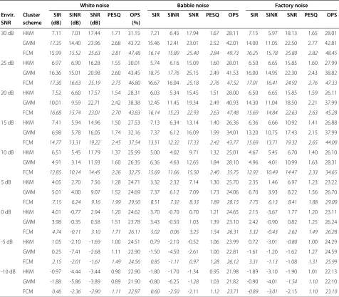
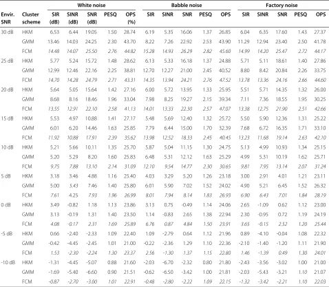
The effect of background noise was then evaluated for the BSS system in the presence of white, babble and factory noise, added to the mixtures as described in section 4.1. The numerical results are shown in Tables 3, 4 and 5 for a range of reverberation times, with similar trends reported for all types of corrupting noise. To provide a fair com-parison against the reverberation-free case in Figure 2, the SIR gain is reported. However, for the SINR and SNR, the absolute measured ratio at the output is provided.

(11)

Figure 2BSS results in reverberant and noise-free conditions.Source separation results compare three clustering techniques for mask estimation (HKM, GMM and FCM). Performance results are given with respect to SIR improvement (dB), where the average input SIR≈ −4.20 dB. The error bars denote the standard deviation.

as previously observed in the separation results of section 4.3.2, the GMM mask estimation ability signif-icantly declines with the introduction of more adverse conditions. For example, in the case of babble noise at a reverberation time of 128 ms, when the SNR is decreased from 25 to 20 dB we note a difference in SIR of almost 5 dB. However, the HKM has a difference of less than 1 dB, and the FCM of just 0.34 dB. Additionally, as was previ-ously observed in the noise-free experiments (Figure 2), the GMM occasionally performs below that of the HKM clustering at the higher reverberation time of 300 ms.

The performance of the SINR is akin to the SIR across all room reverberations and environmental SNRs. To gain an appreciation of any possible noise suppression charac-teristics of the MENUET and its modifications using the GMM/FCM, the SNR was measured and then averaged for all the recovered source signals. The results are gen-erally as expected, with a decrease in gain as the level of noise and reverberation time increase. However, as pre-viously observed, there is often a notable decline in the performance of the GMM as the SNR drops below 20 dB, and/or the room reverberation is increased.

The isolation of the effects of reverberation and noise can be observed in Table 3 when the room reverberation is set to null. The effects of noise alone appear to have less of an impact upon separation ability than the reverbera-tion for the FCM clustering; for example, when the SNR is varied from 30 to 10 dB, there is a change in SIR gain of between 3 and 5 dB, with just a 1 dB change in the case

of babble noise. However, when comparing the SIR gains for the same SNRs across different reverberation times, there are significant differences especially at the reverber-ation time of RT60 = 300 ms. For example, for the case

of corrupting babble noise, for RT60 =0 ms the recorded

SIR was 16.14 dB, whereas when RT60 = 300 ms the SIR

drops to 11.28 dB.

The PESQ was then evaluated on the recovered signals to provide a measure for the perceptual quality of the recovered source estimates. A general decrease in PESQ with an increase in adversity of the conditions is noted, with the FCM for mask estimation yielding the highest scores. The effect of environmental SNR appears to be more detrimental than that of reverberation; for example, in the case of babble noise, the measured PESQ for the FCM method at a reverberation time of 0 ms and SNR of 30 dB is 2.84. When the room reverberation is increased to 300 ms, the measured PESQ is 2.50. However, when the reverberation is maintained at 0 ms and the SNR is decreased to 0 dB, a PESQ is measured at 1.54. This reduc-tion in PESQ is likely due to the decrease in the target sig-nal amplitude and degraded time alignment in such noisy conditions, which leads to a source estimate of poorer quality.

(12)

Table 3 Source separation results in an anechoic enclosure (cf. Figure 1) with background noise

White noise Babble noise Factory noise

Envir. Cluster SIR SINR SNR PESQ OPS SIR SINR SNR PESQ OPS SIR SINR SNR PESQ OPS

SNR scheme (dB) (dB) (dB) (%)

30 dB HKM 7.11 7.01 17.44 1.71 31.15 7.21 6.45 17.94 1.67 28.11 7.15 5.97 18.13 1.65 28.01

GMM 17.35 14.40 23.96 2.68 43.72 15.46 12.41 23.01 2.52 42.01 14.00 11.05 22.50 2.77 42.81

FCM 15.99 15.52 25.63 2.81 47.48 16.14 15.89 25.40 2.84 49.73 16.25 15.78 25.80 2.82 48.45

25 dB HKM 6.97 6.90 16.28 1.55 30.01 5.74 6.16 15.09 1.60 28.01 6.50 6.65 15.85 1.60 27.99

GMM 16.36 15.01 20.98 2.60 43.45 18.75 17.76 25.15 2.49 41.53 16.00 14.95 22.30 2.43 38.82

FCM 17.30 16.63 25.19 2.75 46.80 16.67 16.04 25.18 2.76 47.52 17.01 16.41 24.92 2.76 47.33

20 dB HKM 7.52 6.60 17.57 1.54 28.31 6.03 5.34 15.45 1.51 28.00 6.50 6.65 15.85 1.59 26.11

GMM 10.01 9.59 22.71 2.42 38.38 12.45 11.45 19.34 2.49 40.93 14.30 11.04 18.50 2.21 37.99

FCM 16.68 15.74 23.01 2.70 43.83 16.14 15.23 22.93 2.63 47.48 15.69 14.84 22.63 2.63 45.28

15 dB HKM 7.41 5.94 14.96 1.50 27.53 7.13 6.34 13.14 1.40 26.36 6.36 6.66 10.92 1.41 26.88

GMM 6.98 5.78 16.05 1.74 32.16 7.37 6.12 16.09 1.99 34.01 13.20 10.75 17.43 2.15 37.99

FCM 14.77 13.31 19.22 2.45 37.54 13.51 12.32 17.33 2.42 43.77 15.69 13.71 19.32 2.65 44.00

10 dB HKM 6.51 5.45 11.79 1.37 25.99 5.00 4.02 9.71 1.32 25.01 4.67 5.45 6.70 1.40 26.10

GMM 4.91 3.14 11.93 1.60 26.35 6.36 4.63 12.65 1.84 28.10 4.96 4.01 10.99 1.63 28.31

FCM 12.85 10.14 14.45 2.26 32.75 15.69 11.66 15.50 2.40 35.75 12.92 10.49 14.47 2.33 34.65

5 dB HKM 4.05 2.70 7.56 1.28 24.71 3.32 2.32 7.14 1.30 25.70 2.35 1.46 6.97 1.23 23.22

GMM 5.01 4.00 9.07 1.52 24.69 7.37 6.12 7.09 1.73 24.06 6.70 3.93 8.22 1.56 26.70

FCM 7.15 6.24 9.16 1.99 29.50 8.51 7.32 8.33 1.89 28.15 7.75 6.13 8.41 1.88 29.00

0 dB HKM 4.01 -0.77 2.94 1.20 24.62 3.70 -0.70 0.70 1.21 24.65 2.15 -3.67 1.77 1.20 23.11

GMM 3.98 -0.35 0.58 1.51 23.78 3.43 -0.50 1.03 1.39 23.10 2.42 -0.90 0.82 1.25 26.24

FCM 4.74 -0.11 3.10 1.71 26.11 5.02 0.06 3.25 1.54 26.31 5.32 -0.43 2.62 1.49 26.28

-5 dB HKM 1.05 -2.10 -1.69 1.00 24.51 0.79 -2.10 -0.52 1.06 23.99 0.72 -3.01 -0.80 1.00 24.29

GMM 0.25 -7.41 -2.68 1.11 22.90 -1.50 -4.50 -2.61 1.00 22.81 -1.61 -1.20 -1.62 1.27 24.59

FCM 2.15 -2.01 -1.61 1.49 24.56 0.85 -1.11 0.97 1.28 26.12 3.31 -1.13 -1.08 1.31 25.99

-10 dB HKM -0.97 -4.44 -3.44 0.90 22.90 -1.80 -1.70 -1.34 0.95 21.98 -1.89 -3.10 -1.90 1.01 22.13

GMM -1.88 -5.86 -3.89 0.89 21.90 -0.80 -6.25 -1.28 1.03 21.82 -0.90 -4.01 -1.54 1.10 22.10

FCM 0.46 -2.36 -2.90 1.11 22.97 0.60 -2.50 -2.11 1.12 23.71 -0.89 -3.01 -2.15 1.10 23.10

The room reverberation is set to null. The HKM, GMM and FCM clustering algorithms are compared for TF mask estimation using the performance metrics of SIR gain, SINR and SNR as defined in section 4.2. The highest achieved ratio for each acoustic condition is denoted in italics.

also, the FCM demonstrated its superiority over the HKM and GMM clustering techniques.

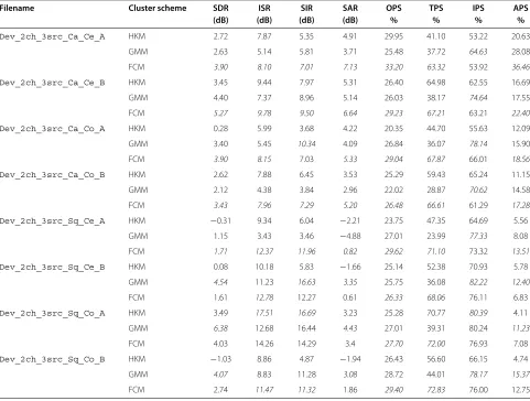
4.3.4 SiSEC 2010 Data

The proposed method was then evaluated with publicly available benchmark data of the SiSEC 2010 [56]. The development data (dev.zip) in “Source separation in the presence of real-world background noise” data sets was used. In this data set, two microphones were spaced at 8.6 cm, and noise signals were recorded in real-world noise environments: ‘Cafeteria’ (Ca) and ‘Square’ (Sq). The ‘Cafeteria’ environment was stated as reverberant (with an unspecified reverberation time), whereas the ‘Square’ had little or no reverberation [56]. The noise sig-nals were recorded at two different positions within the

environment, center (Ce; where noise is more isotropic), and corner (Co; where noise may not be very isotropic) [56]. For each of the noise environments, two differ-ent locations of the same environmdiffer-ent were considered (AandB).

The recordings were 10 s long, with mixed English and Japanese utterances of both genders. The original record-ings were sampled at 16 kHz; however, it was empirically determined that a downsample to 8 kHz resulted in better separation for all methods tested. This can be attributed to the reduced effects of spatial aliasing at the lower sampling frequency.

(13)

Table 4 Source separation results in a reverberant enclosure (cf. Figure 1) with background noise

30 dB HKM 6.53 6.44 19.05 1.50 28.74 6.19 5.35 16.06 1.37 26.85 6.04 6.35 17.60 1.43 27.37

GMM 13.46 14.03 24.25 2.30 43.70 8.22 7.26 22.92 2.53 43.90 11.29 12.94 23.40 2.50 41.78

FCM 14.48 14.07 25.50 2.76 44.82 15.28 14.93 26.29 2.82 45.60 14.99 14.20 25.47 2.72 44.17

25 dB HKM 5.77 5.24 15.72 1.48 28.62 6.13 5.33 16.18 1.37 24.88 5.71 5.11 18.61 1.40 27.86

GMM 12.99 12.46 22.16 2.25 38.81 12.70 12.27 21.00 2.45 40.52 8.80 8.42 20.84 2.26 33.75

FCM 14.70 14.28 24.79 2.71 43.31 14.35 13.94 24.21 2.76 47.52 13.78 13.36 24.16 2.66 44.60

20 dB HKM 5.64 5.05 15.64 1.42 27.16 6.00 5.72 13.95 1.33 25.95 5.51 5.71 14.35 1.32 26.00

GMM 8.68 8.16 18.46 1.96 33.04 7.98 8.25 19.27 2.15 39.34 7.11 7.36 18.55 1.95 30.25

FCM 13.55 12.91 22.10 2.58 41.13 14.01 13.33 22.30 2.57 47.07 13.38 12.75 21.90 2.51 42.66

15 dB HKM 5.53 4.97 10.88 1.41 27.17 5.48 5.69 12.40 1.32 25.72 5.50 5.90 12.36 1.31 25.22

GMM 6.01 6.20 14.46 1.63 25.85 7.79 6.44 15.00 1.70 32.39 7.68 6.72 16.35 1.71 33.10

FCM 11.92 10.88 17.91 2.39 35.62 13.98 12.52 18.33 2.45 40.45 13.23 11.68 19.14 2.63 42.10

10 dB HKM 5.21 5.66 10.11 1.35 25.70 5.87 5.04 11.15 1.30 24.75 5.13 4.99 10.93 1.34 25.15

GMM 5.20 5.29 8.20 1.60 25.83 6.48 5.31 12.12 1.63 25.29 4.99 5.31 10.19 1.62 25.71

FCM 9.75 7.88 13.10 2.14 31.09 12.10 9.54 14.77 2.30 30.65 9.81 7.95 13.14 2.07 31.24

5 dB HKM 3.18 3.46 4.88 1.16 25.40 4.03 3.29 5.20 1.26 23.18 3.00 2.91 4.01 1.21 23.11

GMM 5.00 5.43 7.46 1.40 25.80 6.01 5.90 7.02 1.52 24.02 4.90 5.21 6.45 1.52 26.32

FCM 7.61 4.25 7.93 1.96 26.99 8.01 7.94 8.14 1.83 26.93 6.90 6.43 7.01 1.84 28.19

0 dB HKM 3.49 -0.82 1.18 1.13 23.86 3.13 0.75 -0.49 1.14 24.06 2.65 -1.09 0.62 1.12 23.00

GMM 3.13 -0.19 1.31 1.40 23.50 1.14 -0.83 2.65 1.38 22.94 2.30 -0.95 0.72 1.19 24.19

FCM 4.08 -0.17 2.31 1.69 25.89 6.76 0.87 4.84 1.50 23.91 3.65 -0.15 2.52 1.20 25.44

-5 dB HKM 0.66 -2.40 -2.33 1.09 22.40 1.09 -2.79 0.64 1.12 21.96 0.89 -4.10 -0.04 1.08 22.32

GMM -0.42 -4.45 -2.45 1.01 21.00 -0.22 -2.36 1.29 1.10 22.36 -2.10 -1.40 -1.20 1.11 21.90

FCM 1.53 -2.30 -2.24 1.30 23.37 2.56 -1.30 1.37 1.15 22.80 1.46 -1.39 0.49 1.30 24.01

-10 dB HKM -1.31 -4.45 -5.07 0.88 21.60 -2.03 -6.70 -2.32 0.80 21.80 -2.43 -3.56 -3.02 1.00 21.00

GMM -1.69 -5.40 -6.60 0.90 21.51 -0.62 -6.50 -3.42 1.00 21.81 -2.03 -5.43 -3.21 1.10 21.07

FCM -0.87 -2.70 -3.00 1.01 22.91 -0.48 -2.80 -2.22 1.09 22.15 -1.32 -3.42 -2.21 1.10 22.03

The room reverberation is set to RT60= 128 ms. The HKM, GMM and FCM clustering algorithms are compared for TF mask estimation using the performance metrics of SIR gain, SINR and SNR as defined in section 4.2. The highest achieved ratio for each acoustic condition is denoted in italics.

task was used. The estimated source image ˆsmn(t) is

decomposed as

ˆ

smn(t)=simgmn(t)+espatmn(t)+einterfmn (t)+eartifmn(t). (30)

Three energy ratios, the source image to spatial distortion ratio (ISR), signal to interference ratio (SIR) and the signal to artifact ratio (SAR), then measure the amount of spa-tial distortion, interference and artifacts in the recovered source estimates. These are expressed in dB as [52]

ISRn=10log10 M m=1 ts

img mn(t)2 M

m=1 te spat mn(t)2

(31)

SIRn=10log10 M m=1 t(s

img

m=1 teinterfmn (t)2

(32)

SARn=10log10 M m=1 t(s

img

mn(t)+espatmn(t)+einterfmn (t))2 M

m=1 teartifmn(t)2

.

(33)

The total error is captured in the signal-to-distortion ratio (SDR)

SDRn=10log10

M m=1 ts

img mn(t)2 M

m=1 t(e spat

mn(t)+einterfmn (t)+eartifmn(t))2 .

(14)

Table 5 Source separation results in a reverberant enclosure (cf. Figure 1) with background noise

30 dB HKM 5.27 5.91 20.29 1.34 22.50 5.10 6.23 20.84 1.36 21.48 5.12 5.89 22.53 1.34 24.45

GMM 6.87 7.71 22.81 1.83 30.15 6.64 7.57 23.52 1.81 21.83 6.34 6.22 22.86 1.71 20.30

FCM 11.62 11.49 24.66 2.42 35.88 11.28 12.12 25.32 2.50 35.46 11.56 9.45 25.12 2.36 35.63

25 dB HKM 5.61 5.97 15.90 1.35 22.90 5.83 5.32 16.76 1.34 21.44 5.23 4.73 15.42 1.33 23.92

GMM 6.60 6.37 20.33 1.81 23.63 6.27 6.07 20.32 1.80 23.91 6.07 5.94 20.31 1.70 20.68

FCM 9.01 8.76 23.68 2.40 35.10 10.26 10.04 24.05 2.36 35.40 9.42 9.25 24.08 2.30 35.84

20 dB HKM 5.46 5.69 14.01 1.35 23.18 5.80 5.25 14.30 1.33 23.30 4.98 4.49 13.75 1.28 23.16

GMM 6.40 5.96 16.67 1.68 23.64 6.15 5.87 18.34 1.67 22.52 6.26 6.01 16.61 1.66 20.70

FCM 8.05 7.77 21.05 2.34 32.31 10.08 9.64 21.69 2.35 34.64 9.22 8.90 21.36 2.27 33.76

15 dB HKM 5.77 5.11 12.85 1.36 23.01 4.16 4.86 13.68 1.32 22.03 5.81 5.88 12.46 1.34 22.54

GMM 6.11 5.35 12.69 1.61 23.51 5.28 5.82 12.35 1.60 21.18 4.70 4.28 13.75 1.59 23.14

FCM 7.12 6.43 16.93 2.21 28.55 7.18 6.66 17.85 2.42 33.34 8.52 7.59 17.94 2.21 32.91

10 dB HKM 4.46 4.90 10.03 1.31 23.80 4.72 4.91 10.94 1.30 22.13 4.67 4.47 10.26 1.30 22.44

GMM 4.01 4.21 9.64 1.58 23.50 5.32 4.61 11.55 1.58 22.16 5.12 4.40 8.79 1.60 22.34

FCM 7.97 6.39 12.29 1.90 26.59 8.65 7.05 12.39 2.10 27.31 6.97 6.85 12.35 1.96 27.11

5 dB HKM 3.09 3.08 5.61 1.14 22.45 3.10 3.71 4.71 1.18 21.51 3.09 2.72 6.45 1.17 22.25

GMM 3.90 3.16 6.26 1.16 22.94 4.65 3.51 5.74 1.40 22.00 4.08 4.91 5.78 1.31 21.05

FCM 6.73 6.37 7.29 1.90 24.82 6.52 5.96 7.39 1.89 24.13 5.55 6.97 7.15 1.81 23.88

0 dB HKM 2.16 -0.60 2.30 1.10 22.01 1.47 -0.34 1.73 0.98 21.03 1.04 -1.70 2.12 0.90 22.24

GMM 1.81 -0.70 1.60 1.04 21.92 -0.46 -0.27 1.70 1.10 22.19 -0.84 -0.64 2.59 1.00 20.57

FCM 2.60 -0.35 2.54 1.15 24.00 2.72 -0.25 2.38 1.14 23.57 2.58 -0.62 2.51 1.13 22.86

-5 dB HKM 0.46 -2.74 -2.71 1.09 21.69 -0.49 -3.29 -0.79 0.92 20.56 -1.19 -2.81 0.80 1.07 21.22

GMM -0.58 -4.59 -0.43 1.02 21.73 -1.01 -3.29 -0.36 0.91 20.57 -1.20 -2.34 1.64 0.92 20.49

FCM 0.88 -2.62 -1.67 1.10 21.93 0.78 -0.42 -0.41 1.12 21.00 1.52 -1.82 2.08 1.10 21.91

-10 dB HKM -2.54 -5.58 -3.34 0.85 21.05 -2.48 -5.13 -3.10 0.79 19.83 -2.34 -4.01 -3.10 0.97 20.37

GMM -1.59 -6.76 -3.71 0.89 21.04 -1.01 -5.64 -1.91 0.90 20.29 -2.13 -5.32 -3.98 0.90 21.05

FCM -1.55 -2.51 -3.14 1.00 21.17 -0.64 -4.16 -1.42 1.01 21.01 -1.57 -3.30 -2.13 0.99 21.09

The room reverberation is set to RT60= 300 ms. The HKM, GMM and FCM clustering algorithms are compared for TF mask estimation using the performance metrics of SIR gain, SINR and SNR as defined in section 4.2. The highest achieved ratio for each acoustic condition is denoted in italics.

The quality of the source signals were also evaluated with the PEASS toolkit as described in section 4.2.3. How-ever, all four ratios were included: the target-related per-ceptual score (TPS), interference-related perper-ceptual score (IPS), artifact-related perceptual score (APS) and the OPS. The reader is referred to [51] for details.

Table 6 shows the average results per environmental condition, averaged across all available mixtures. This table can easily be compared against the results of the SiSEC 2010, in the table entitled “Average Results

for 2 channels” in [58]. The individual results for

each recording are displayed in Table 7. The reported results are at a similar performance level with those pub-lished in the SiSEC 2010 [58], despite the reduced SAR and APS ratios. An overall decline in performance in

comparison to the simulated evaluations (Tables 3, 4 and 5) can be observed. A likely reason for this is due to the larger sensor spacing (8.6 cm compared to the 4 cm spacing in previous evaluations), as for ideal phase mea-surements, the sensor spacing should be limited to below c/fs, wherecis the velocity of sound andfsis the sampling

frequency [21]. Additionally, the fact that two sensors are used to retrieve the information compared to three, as in section 4.3.3, could contribute to the decrease in per-formance. The reduction of the feature space dimension may have lowered the capability of the clustering algo-rithm, making any clustering performance differences less apparent.

(15)

Table 6 Average separation results for the SiSEC 2010 data

Environment Cluster scheme SDR ISR SIR SAR OPS TPS IPS APS

(dB) (dB) (dB) (dB) % % % %

Cafeteria HKM 2.27 7.80 5.86 4.49 25.50 52.55 59.16 15.14

GMM 3.13 5.59 7.23 3.98 25.10 35.21 72.00 19.03

FCM 4.13 8.50 7.71 6.10 29.50 66.30 61.11 23.70

Square HKM 0.56 11.47 8.36 −0.64 25.15 56.78 70.54 5.05

GMM 4.04 9.04 11.95 1.50 27.12 35.85 79.49 11.77

FCM 2.53 12.72 12.46 1.67 28.26 71.00 75.79 10.03

The average measured output ratio across all three sources, and for all mixtures in the condition, is displayed. The highest achieved ratio is denoted in italics.

however the remaining ratios were not as high as those achieved with the FCM. For example, the OPS was con-sistently at its highest when the FCM was used for mask estimation. Interestingly, the location of the noise source (center or corner) did not appear to have a substan-tial effect on the separation ability. This suggests that the proposed algorithm is robust in both isotropic and non-isotropic noise conditions.

4.4 Discussion

The experimental results presented have demonstrated that the implementation of the FCM clustering for mask estimation with a nonlinear microphone array setup as in the MENUET renders superior separation performance in conditions where reverberation and/or environmental noise exist. The feasibility of the FCM clustering was ini-tially tested on a range of spatial feature vectors in an

Table 7 Separation results for the SiSEC 2010 data

Filename Cluster scheme SDR ISR SIR SAR OPS TPS IPS APS

(dB) (dB) (dB) (dB) % % % %

Dev_2ch_3src_Ca_Ce_A HKM 2.72 7.87 5.35 4.91 29.95 41.10 53.22 20.63

GMM 2.63 5.14 5.81 3.71 25.48 37.72 64.63 28.08

FCM 3.90 8.10 7.01 7.13 33.20 63.32 53.92 36.46

Dev_2ch_3src_Ca_Ce_B HKM 3.45 9.44 7.97 5.31 26.40 64.98 62.55 16.69

GMM 4.40 7.37 8.96 5.14 26.03 38.17 74.64 17.55

FCM 5.27 9.78 9.50 6.64 29.23 67.21 63.21 22.40

Dev_2ch_3src_Ca_Co_A HKM 0.28 5.99 3.68 4.22 20.35 44.70 55.63 12.09

GMM 3.40 5.45 10.34 4.09 26.84 36.07 78.14 15.90

FCM 3.90 8.15 7.03 5.33 29.04 67.87 66.01 18.56