Capturing Word Semantics From Co-occurrences Using Dynamic Mutual Information

(1)

Scholarship at UWindsor

Electronic Theses and Dissertations Theses, Dissertations, and Major Papers

3-10-2019

Capturing Word Semantics From Co-occurrences Using Dynamic

Mutual Information

Yaxin Li

University of Windsor

Follow this and additional works at: https://scholar.uwindsor.ca/etd

Recommended Citation Recommended Citation

Li, Yaxin, "Capturing Word Semantics From Co-occurrences Using Dynamic Mutual Information" (2019). Electronic Theses and Dissertations. 7644.

https://scholar.uwindsor.ca/etd/7644

This online database contains the full-text of PhD dissertations and Masters’ theses of University of Windsor students from 1954 forward. These documents are made available for personal study and research purposes only, in accordance with the Canadian Copyright Act and the Creative Commons license—CC BY-NC-ND (Attribution, Non-Commercial, No Derivative Works). Under this license, works must always be attributed to the copyright holder (original author), cannot be used for any commercial purposes, and may not be altered. Any other use would require the permission of the copyright holder. Students may inquire about withdrawing their dissertation and/or thesis from this database. For additional inquiries, please contact the repository administrator via email

(2)

Co-occurrences Using Dynamic Mutual

Information

By

Yaxin Li

A Thesis

Submitted to the Faculty of Graduate Studies through the School of Computer Science in Partial Fulfillment of the Requirements for

the Degree of Master of Science at the University of Windsor

Windsor, Ontario, Canada

2019

c

(3)

by

Yaxin Li

APPROVED BY:

A. Hussein

Department of Mathematics and Statistics

R. Gras

School of Computer Science

J. Lu, Advisor School of Computer Science

(4)

I hereby certify that I am the sole author of this thesis and that no part of this thesis has

been published or submitted for publication.

I certify that, to the best of my knowledge, my thesis does not infringe upon anyones

copyright nor violate any proprietary rights and that any ideas, techniques, quotations, or

any other material from the work of other people included in my thesis, published or

oth-erwise, are fully acknowledged in accordance with the standard referencing practices.

Fur-thermore, to the extent that I have included copyrighted material that surpasses the bounds

of fair dealing within the meaning of the Canada Copyright Act, I certify that I have

ob-tained a written permission from the copyright owner(s) to include such material(s) in my

thesis and have included copies of such copyright clearances to my appendix.

I declare that this is a true copy of my thesis, including any final revisions, as approved

by my thesis committee and the Graduate Studies office, and that this thesis has not been

(5)

Semantic relations between words are crucial for information retrieval and natural

lan-guage processing tasks. Distributional representations are based on word co-occurrence,

and have been proven successful. Recent neural network approaches such as Word2vec

and Glove are all derived from co-occurrence information. In particular, they are based on

Shifted Positive Pointwise Mutual Information (SPPMI). In SPPMI, PMI values are shifted

uniformly by a constant, which is typically five. Although SPPMI is effective in

prac-tice, it lacks theoretical explanation, and has space for improvement. Intuitively, shifting

is to remove co-occurrence pairs that could have co-occurred due to randomness, i.e., the

pairs whose expected co-occurrence count is close to its observed appearances. We

pro-pose a new shifting scheme, called Dynamic Mutual Information (DMI), where the shifting

is based on the variance of co-occurrences and Chebyshev’s Inequality. Intuitively, DMI

shifts more aggressively for rare word pairs. We demonstrate that DMI outperforms the

(6)

I would like to express my sincere appreciation to my supervisor Dr. Jianguo Lu for his

constant guidance and encouragement during my whole Master’s period at the University

of Windsor. Without his help, this thesis would not have been possible.

I would also like to express my appreciation to my thesis committee members Dr. Robin

Gras and Dr. Abdulkadir Hussein. Thank you all for your valuable suggestions to this

thesis.

Last but not least, I want to express my gratitude to my parents and my friends who are

(7)

DECLARATION OF ORIGINALITY III

ABSTRACT IV

ACKNOWLEDGEMENTS V

LIST OF TABLES VIII

LIST OF FIGURES XI

1 Introduction 1

2 Review of The Literature 4

2.1 Different Co-occurrences . . . 4

2.2 Distributional Models . . . 5

2.3 Neural Network Models . . . 6

2.4 Matrix Factorization and Neural Network Models . . . 7

3 Co-occurrence 9 3.1 Window Sytles . . . 10

3.1.1 Basic Window . . . 10

3.1.2 Word2vec Window . . . 11

3.1.3 Weighted Window . . . 14

3.1.4 Relationship Between Different Window Styles . . . 14

3.2 Expected Co-occurrences . . . 23

3.2.1 From the Perspective of Windows . . . 25

3.2.2 From the Perspective of Word Pairs . . . 25

3.3 Fij andFˆij . . . 27

3.3.1 Mean, variance and rse ofFij . . . 27

3.3.2 Mean, variance and rse ofFˆij . . . 28

4 Pointwise Mutual Information (PMI) 32 4.1 PMI andFˆij . . . 32

4.2 Shifted Positive PMI (SPPMI) . . . 33

4.2.1 Shifted PMI . . . 33

4.2.2 SPPMI . . . 34

4.2.3 Why Positive . . . 35

4.3 Singular Value Decomposition (SVD) . . . 36

5 Dynamic Mutual Information (DMI) 38 5.1 Variance ofr . . . 38

(8)

6.2 Word Pair Selection . . . 48

6.3 Values of Mutual Informations . . . 49

6.4 Word Vectors . . . 61

7 Experiments 62 7.1 Data Sets . . . 62

7.1.1 Corpus . . . 62

7.1.2 Test Data Sets . . . 63

7.2 Word Similarity Tasks . . . 64

7.2.1 Choosing Parameters for SPPMI . . . 65

7.2.2 Word2vec Settings . . . 67

7.2.3 Results . . . 68

7.3 Statistical Significance on Word Similarity Tasks . . . 78

7.4 Word Analogy Tasks . . . 79

7.5 Implementation . . . 83

7.5.1 Space Complexity . . . 84

7.5.2 Word Pair Collection . . . 84

7.5.3 Scalability . . . 85

7.6 Examples of SPPMI and DMI . . . 86

8 Conclusions 90

REFERENCES 93

(9)

1 Notations. . . 9

2 A simple text corpus . . . 10

3 Steps of collecting word pairs using basic windows . . . 12

4 The co-occurrence matrix using basic window . . . 12

5 Steps of collecting word pairs using Word2vec window . . . 13

6 The co-occurrence matrix using word2vec window . . . 14

7 Steps of collecting word pairs using weighted window . . . 15

8 The co-occurrence matrix using weighted window . . . 15

9 Frequencies of Word Pairs Using Different Windows. The window size is 6. The data set is Wiki-100. . . 20

12 Most frequent word pairs using different windows. The window size is 6. The data set is Wiki-100. . . 23

15 A samll PMI matrix. . . 35

16 Frequency ofFij after Shifting on Wiki-100. . . 48

17 PPMI, SPPMI and DMI of word pairs whoseFij >10,000. Dataset: Wiki-100. . . 50

(10)

Fij <2,000. Dataset: Wiki-100. . . 52

20 PPMI, SPPMI and DMI of 100 randomly selected word pairs whose500 < Fij <600. Dataset: Wiki-100. . . 53

24 PPMI, SPPMI and DMI of 100 randomly selected word pairs whose 0 < Fij <5. Dataset: Wiki-100. . . 57

25 Word pairs in Table 17, 18, 19, 20, 21, 22, 23, 24 when only DMI=0 or only SPPMI=0. Part I. . . 58

26 Word pairs in Table 17, 18, 19, 20, 21, 22, 23, 24 when only DMI=0 or only SPPMI=0. Part II. . . 59

27 Word pairs in Table 17, 18, 19, 20, 21, 22, 23, 24 when only DMI=0 or only SPPMI=0. Part III. . . 60

28 Corpora Statistics . . . 63

29 Test Sets Statistics . . . 64

30 A sample of word analogy test set. . . 64

31 An example of Spearman’s correlation. . . 65

32 The word similarity results on different corpus.Min-count=0 . . . 69

34 Improvements in WS353. Dataset: Wiki-1000. . . 74

35 Improvements in Mturk. Dataset: Wiki-1000. . . 76

36 Improvements in Men. Dataset: Wiki-1000 . . . 77

37 Significance test on the improvements . . . 79

(11)

(12)

1 The variance ofras theFˆij increases. . . 2

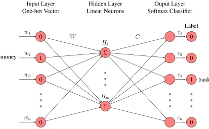
2 The architecture of Word2vec Skip-Gram model, and the current word pair is(money, bank). . . 6

3 Three kinds of co-occurrences. The window size is 6. . . 10

4 Distribution of co-occurrences using different windows on 3 datasets. Stop words are included. . . 17

5 Distribution of co-occurrences using different windows on 3 datasets. Stop words are removed. . . 18

6 Mean ofFij whenFˆij is between 0 and 300. . . 28

7 Variance ofFij whenFˆij is between 0 and 300. . . 29

8 Rse ofFij whenFˆij is between 0 and 300. . . 29

9 Mean ofFˆij whenFij is between 0 and 500. . . 30

10 Variance ofFˆij whenFij is between 0 and 500. . . 31

11 Rse ofFˆij whenFij is between 0 and 500. . . 31

12 Vector of word “percent” from PMI, SPMI and DMI matrix. . . 34

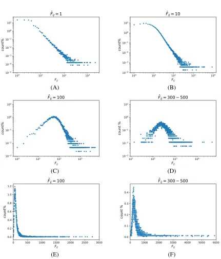
13 The distribution ofFij whenFˆij = 1,10,100 and300−500. (E) and (F) are another versions of (C) and (D) without loglog plot. The data set is Wiki-100. . . 40

(13)

18 Mean ofrasFij increases on different data sets. . . 47

19 Mean of different MIs whenFij = 1−500. . . 50

20 The influence of different shifting values in SPPMI on Wiki-100. . . 66

21 The influence of different shifting values in SPPMI on Wiki-1000. . . 66

22 The influence of different shifting values in SPPMI on Reuters. . . 67

23 The word similarity results on different corpus. . . 71

25 The average number of non-zero elements in the word vector as the word frequency increases . . . 75

26 Word pairs with SPPMI and DMI representations in 2D plot. The dimen-sion is reduced by PCA, the dataset is Wiki-1000 . . . 87

(14)

Introduction

Semantic relations between words is crucial for information retrieval and natural language

processing problems, such as entity extraction [31], word similarity and analogy [18, 13].

Word co-occurrence has been widely used for extracting word semantics and

representa-tions.

The most simple word distributional representation is the co-occurrence raw count

ma-trix in HAL [16]. Each row in the co-occurrence mama-trix is used to represent a word

vec-tor. COALS [25] improves HAL model by ignoring the left-right distinction in word pair

collection, replacing the raw co-occurrence count with Pearson’s Correlation coefficient

between two words. More importantly, it removes negative values in the matrix. It

outper-forms HAL on word similarity tasks and word classification tasks. More generally, more

measures of word association can be applied in the matrix, each cell of which is the word

association between two words.

The first influential research on word association norms [21] is based on empirical

estimates. This study measured 200 words by asking subjects from grade school to

col-lege to write down a word after one word is given. As more computational resources are

available, we can analyse the word relationships on large corpora, and more measures are

proposed to represent word associations, such as Pointwise Mutual Information (PMI) [6],

log-likelihood ratio [8] andχ2 measure [11].

Recent neural network approaches to word representation learning, such as Word2Vec,

are all based on word co-occurrences within a text window [19]. Those approaches are also

tied to more traditional measurement of co-occurrence, e.g., using pointwise mutual

(15)

0 50 100 150 200 250 300

̂F

ij 1.0

1.5 2.0 2.5 3.0 3.5 4.0 4.5

σr

variancêof̂r

FIGURE 1: The variance ofras theFˆij increases.

PMI matrix, of which each cell is the PMI of the corresponding word pair shifted by a

con-stant, typicallylog 5. Moreover, they found that, if all the negative values are nullified, the

word representations generated from shifted positive PMI(SPPMI) matrix can also achieve

great performance on different tasks.

PMI measures the logarithm of the ratio r between the co-occurrence count and the

expected count, assuming that two wordsi andj are independent. P M I(i, j) = logr =

logFij/Fˆij. If the co-occurrence count is larger than expected, the ratior will be larger

than 1, thus its P M I(i, j) > 0. This means that wordsi andj co-occur more often than

randomness, and they are associated positively. Although P M I(i, j) > 0indicates that

x and y associate positively, [6] observed that ”genuine“ association requiresI(i, j) 0.

P M I(i, j)(the logarithm in this work is based on 2 ) should be greater than 3 by manually

inspecting word pairs and MI values. Associations with MI value less than 3 are found to

be generally not interesting. [14] shows a similar value (P M I = log₂5 = 2.3), they shift

all the ratios by 5.

SPPMI nullifies unreliable values, i.e., the values less than log 5 or ratios less than 5,

in a PMI matrix. Intuitively, the ratio is unreliable for rare words. However, for popular

words, i.e., whenfi andfj are large, the ratio becomes more reliable. More formally, the

variance of the ratio changes over the frequency of the words, which is shown in Figure 1.

(16)

ratio.

This paper proposes Dynamic Mutual Information (DMI), where the PMI of each word

is dynamically shifted according to the variance of ratior. We show that DMI outperforms

SPPMI on different word similarity test sets, and an improved Steiger’s test [24] is used to

compute how significant the improvements of our DMI against are SPPMI, and most of the

(17)

Review of The Literature

This chapter reviews related research works about word co-occurrences and different word

representation models.

2.1 Different Co-occurrences

Lexical co-occurrence is widely used to construct semantic spaces. Almost all the word

representation models are based on word co-occurrences, and they belongs to two main

categories: one is the distributional model and the other is the neural network based model.

The distributional models [16, 25, 14] are derived from the co-occurrence matrix, and the

popular neural network based models also utilize the information of word co-occurrences.

There are different word co-occurrences that are commonly used. The first and simplest

is to use a window of lengthkthat moves across the corpus: every two words in this window

is considered one co-occurrence count. Another version of this window is that, for every

word in the corpus, its neighbor word will receive a weighted count of k −1 if they are adjacent,k−2if it is 2 words from the word, and so forth. In Section 3.1, we will discuss how different windows capture the co-occurrence between two words, and prove that these

windows are roughly the same. There are also some variations of this kind of window, but

they are all based on the same idea that closer words have higher co-occurrence weights.

In distributional models, these word co-occurrences can form a co-occurrence matrix,

of which each row and each column represents one word in the vocabulary and each

el-ement is the co-occurrence count of two corresponding words. However, it is impossible

(18)

co-occurrence matrix is extremely sparse. [29] proposed Neural Latent Relational Analysis

(NLRA) to relieve the sparseness problem, and can obtain the embeddings of word pairs

that do not co-occur in the corpus.

Apart from word pair co-occurrences, k-way word co-occurrences [4], which is

gen-erated from random walk are also used. Associated words do not always occur as pairs

in the sentences, in natural languages multiple words can be related and co-occurring in

the context. By splitting the sentences into word pairs, we lose some information. For

example, in the sentenceThe University of South California is located in Los Angeles, we

can have one three-way co-occurrence (University, South, California), if it is split into 3

word pairs(University,South),(South, California)and(South, University), the information

is incomplete.

Moreover, [33] introduced ngram statistics to explore more information in the source

text. They use “ngram-ngram” type of co-occurrences instead of “word-word”. To solve

the problems brought by ngrams, new methods are proposed to build the co-occurrence

matrix more efficiently.

2.2 Distributional Models

The most explicit model is Hyperspace Analogue to Language(HAL) [16], which uses

word co-occurrence count directly as the word vector. Word co-occurrences are recorded

by moving a window over the corpus in one word increment, and for each word pair within

a window, their co-occurring counts are weighted inversely proportional to the number of

other words separating them. Also, the word pair is direction sensitive, which means word

pairs(x, y)and(y, x)are different. In this way, the co-occurrence matrix is not symmetric

and the representation of theith word is the concatenation of theith column and theith row.

In the end, they use the Minkowski family of distance metrics to measure the similarity of

different words. HAL gives a simple way of finding the word representations and yields

good results. However, it suffers from the extremely high frequency of popular words or

stop words, because they use raw counts directly.

(19)

..

.

0

1

0

0 money

..

.

Σ

..

.

..

.

bank 0

0

1

0

w1

w2

w3

wn

H1

Hm

c1

c2

c3

cn Input Layer

One-hot Vector

Hidden Layer Linear Neurons

Ouput Layer Softmax Classifier

Label

W C

FIGURE 2: The architecture of Word2vec Skip-Gram model, and the current word pair is

(money, bank).

solved the problems caused by raw counts. Besides, it used a similar window, but ignores

the left-right distinction between word pairs. Another improvement is discarding the

nega-tive values, which greatly boosts the performance of word vectors. In the end, each row of

the matrix is the representation of the corresponding word, and COALS measures the word

similarity with correlations.

In practice, the co-occurrence count in the matrix can be replaced with different

mea-sures of word association, such as Pointwise Mutual Information (PMI) [6], log-likelihood

ratio [8] andχ2 _{measure [11].}

2.3 Neural Network Models

Neural network based models are becoming popular in discovering word semantic

rela-tions. They use neural network’s internal word vectors to represent the word [3, 7], and the

most popular models are Word2vec [19, 18] and GloVe [22]. These models are also using

word co-occurrence information to create word embedding.

(20)

and several context wordscj which are within k tokens to each side of the center word. As

the window moves, each word can be a center word or context word and the actual window

size will be shrunk by a random integer r (0≤r≤k−1). Thus, the closer a context word is to the center word, the higher probability the context word can be considered as a word

pair with the center word. Note that the window is the same as that used in COALS.

Simi-larly, GloVe also gives higher weights to the closer context word, but a different weighting

scheme is applied, less weights are given to the farther context word than that in word2vec

window.

Figure 2 shows the simple architecture of Word2vec Skip-Gram model. The input layer

is the one-hot vector of the center word “money”, which means the element in “bank”

position is 1 and all the other elements are 0s. The hidden layer consists of m linear

neurons andmis the dimension of word embeddings. In the output layer, it uses softmax

classifier to predict the probability of each word being its context, and its ground truth is

“bank” in this case. Moreover, Word2vec uses stochastic gradient descent to minimize the

loss function. In the end, the input vectorsW are used as word representations and output

vectorsCare the context vector. It is reported that the word vectors from Word2vec have

a more promising performance than any other neural network models. Glove is similar to

Word2vec, but it takes the global word statistics into account.

Compared with distributional models, neural network based models project the word

representations into a very low dimension, usually a few hundred, but the dimension is

much higher in distributional models: it is the size of the vocabulary. The low-dimensional

dense vectors have its advantages in improving the computational efficiency over

distribu-tional models. However, the neural network based models have several hyper parameters

and it suffers from parameter tuning. The parameters have to be changed for different

corpus, and this process is time-consuming.

2.4 Matrix Factorization and Neural Network Models

[14] related the neural network models with the traditional distributional models. They

(21)

a shifted Pointwise Mutual Information (PMI) matrix, of which each cell is the PMI

val-ue between two words shifted by a constant. Furthermore, in order to take the advantage

of dense low-dimensional word vectors, [15] proposed to use Singular Value

Decompo-sition(SVD) to find the optimal rankd factorization of the shifted PMI matrix to get the

low-dimensional word representations, and gave some suggestions on tuning the hyper

parameters in generating word embeddings. [28] discussed further about all kinds of

pa-rameters in the matrix factorization, and introduced canonical correlation analysis (CCA)

to improve the performance of matrix decompositions. [2] gives a theoretical justification

for PMI based models, as well as hyper parameter choices by proposing a new generative

(22)

Co-occurrence

There are several different methods to calculate the co-occurrences of word pairs [16, 25,

18, 22]. Usually, a window is introduced, and the co-occurrences of every word pair within

one window are recorded. As the window moves across the corpus by one token, a

co-occurrence matrix is formed to record the co-co-occurrence values of every two words in the

corpus. Each column and each row of the matrix represents a unique word in the corpus,

and the value of each cell is the co-occurrence count between two corresponding words.

More formally, suppose that the vocabulary (the set of distinct words) isV ={w1, w2, . . . , w|V|},

and the size of the co-occurrence matrix is|V| × |V|. Given a corpus that consists of a se-quence of words wx1, wx2, . . . , wxn, where xi ∈ {1,2, . . . ,|V|} and n is the number of

tokens in the corpus . Let k be the window size. The notations we are going to use are

listed in Table 1, and we will talk about three popular window styles in collecting word

pairs.

Corpus n Corpus length, i.e., # words in the corpus

V Vocabulary size, # unique words in the corpus

fi Frequency of wordiin corpus

k Window size

N # pairs sampled. N = (n−k)k(k−1)≈nk(k−1)

Pairs Fi # word pairs whose first word is wordwi. Fi =fik(k−1).

Fj # word pairs whose second word is wordwj. Fj =fjk(k−1).

Fij Cooccurrence of word pair(wi, wj)in sampled word pairs

ˆ

Fij Estimated cooccurrence count of wordiandj if they are independent.

ˆ

Fij = FiFj

n =

fifj

n k(k−1).

(23)

how much wood would a woodchuck chuck, if a woodchuck could chuck wood? as much wood as a woodchuck would,if a woodchuck could chuck wood.

TABLE 2: A simple text corpus

...wi−5wi−4wi−3wi−2wi−1wiwi+1wi+2wi+3wi+4wi+5...

(A): Basic Window

1 5

2 5

3 5

4 5

5 5

1 5 2 5 3 5 4 5 5 5

(B): Word2vec Window

1 2 3 4 5 5 4 3 2 1

(C): Weighted Window.

FIGURE 3: Three kinds of co-occurrences. The window size is 6.

3.1 Window Sytles

In this section, we will introduce three most common window styles, and compare the

differences between them by analysing their word pair distributions. In order to make each

method easier to understand, we will give a sample co-occurrence matrix for each window

style using a short text in Table 2.

3.1.1 Basic Window

The basic window is the most straightforward way of collecting word pairs. We move

(24)

considered as one co-occurrence. As the window moves, a co-occurrence matrix is formed.

Even though it ignores the order and position of words, adjacent words have a higher

weight than words lying farther apart. Figure 3(A) shows that, with a window of size 6,

adjacent words(wi−1, wi)has five co-occurrences when the window slides by, while words

four positions apart like(wi−4, wi)has only two co-occurrence.

Some steps of collecting word pairs are shown in 3, and the final co-occurrence matrix is

shown in Table 4. Since we ignore the left-right distinction of word pairs, the co-occurrence

matrix is symmetric, for example, the co-occurrence count of wi andwj is Fij = 5, thus

the value ofith row andj th column is 5, so is the value ofj th row andith column, and

Fji = 5.

For the word pair (a, chuck), they first co-occur in the window(size 6)...much wood

would a woodchuck chuck ..., when the window moves, the following three windows also

contain this pair, so the count increases to 4. Then 3 windows also contain this pair starting

at ...chuck, if a woodchuck could chuck wood..., next, the pair also appears in another 3

windows starting at...would, if a woodchuck could chuck wood.... In total,F(a, chuck) =

4 + 3 + 3 = 10.

Let the corpus length be n, and there are totaln−kwindows if there are no sentence breaks in the corpus, i.e., the sliding window does not restart for each sentence. Since

n k, the total number of windows is approximaten. Within each window, there are k₂ word pairs collected, and because Fij = Fij, we have 2₂k

more co-occurrence count on

the co-occurrence matrix.

3.1.2 Word2vec Window

Word2vec window is a very popular window style in neural network based models. The

length of the window varies as it moves over the sentence. In a dynamic window with size

(25)

Current Window Pairs Count

how much wood would a woodchuck (how much) +1

(how wood) +1

(how would) +1

(how a) +1

(how woodchuck) +1

(much wood) +1

(much would) +1

8 more pairs...

much wood would a woodchuck chuck (much wood) +1

(much would) +1

(much a) +1

(much woodchuck) +1

(much chuck) +1

(wood would) +1

(wood a) +1

8 more pairs...

... ... ...

TABLE 3: Steps of collecting word pairs using basic windows

a as chuck could how if much wood woodchuck would

a 8 9 14 8 1 16 5 12 28 13

as 9 6 5 3 0 2 9 16 7 3

chuck 14 5 2 12 0 9 4 14 16 4

could 8 3 12 0 0 6 2 9 12 2

how 1 0 0 0 0 0 1 1 1 1

if 16 2 9 6 0 0 0 4 16 7

much 5 9 4 2 1 0 0 11 5 3

wood 12 16 14 9 1 4 11 6 12 5

woodchuck 28 7 16 12 1 16 5 12 8 12

would 13 3 4 2 1 7 3 5 12 0

(26)

Center Word

Dynamic Length

Context Word

Word Pair Count

how 3 much (how much) +1

wood (how wood) +1

would (how would) +1

much 5 how (much how) +1

wood (much wood) +1

would (much would) +1

a (much a) +1

woodchuck (much woodchuck) +1

chuck (much chuck) +1

... ... ... ... ...

TABLE 5: Steps of collecting word pairs using Word2vec window

the context word is k_k−₋d₁, which can be illustrated in Figure 3 (B). After collecting the pairs

in the current window, the window moves forward by one token, so does the center word.

For example, the center word in Figure 3 (B) iswi and the center word of the next window

will bewi+1.

Some word collecting steps in Word2vec window are shown in Table 5, and the final

co-occurrence matrix is shown in Table 6. The matrix is supposed to be symmetric because

as the window moves, the current center word can be the context word of the next several

center words, but the matrix is not symmetric due to the dynamically changed window size.

Similar to the basic window style, there are approximate n windows, and within each

window, we collectkco-occurrence count on average due to the probability, which means if

we run Word2vec window(k−1)times, we will collect the same number of co-occurrence counts as that in basic window.

Word2vec window gives a higher probability to the closer words, and it works fine for

the neural network based methods, because the neural network models usually have more

than one iteration(epoch), and the corpus will be scanned several times. In this way, even

the distant word pairs with lower probabilities can be sampled in one of these iterations.

However, such windows were also applied in some count-based models [15], where the

corpus is scanned only once, and if we use dynamic window on a small corpus to count the

word pairs, the relations between distant word pairs will be lost, which leads to degraded

(27)

a 2 2 1 0 1 4 2 3 5 2

as 1 1 1 0 0 0 2 3 1 1

chuck 3 1 0 3 0 2 0 3 4 2

could 2 1 3 0 0 2 1 2 2 0

how 0 0 0 0 0 0 1 1 0 1

if 3 1 2 1 0 0 0 2 2 1

much 2 2 2 1 1 0 0 3 3 2

wood 2 3 4 3 1 2 3 2 3 2

woodchuck 5 0 3 2 0 3 1 2 2 3

would 3 1 1 1 0 1 2 2 3 0

TABLE 6: The co-occurrence matrix using word2vec window

3.1.3 Weighted Window

Another window style is widely used in distributional models [16, 25], and here we call

it weighted window. It used a length k window, and for every word wi in the corpus, its

neighbor word will receive a weighted count ofk−1if they are adjacent,k−2if it is 2 words fromwi, and so forth. The window and the weighting schemes are shown in Figure

3(C). We can see that the weighted window is another version of Word2vec window, and it

replaces the probabilities with the real count to avoid the uncertainty. Whenk = 6, if we

run the Word2vec window 5 times, it should be equal to the weighted window.

Some steps of collecting word pairs are shown in Table 7. After all the pairs are

col-lected, the co-occurrence matrix is in Table 8, where each row represents the center words

and the columns are the context words. Note that, the matrix is symmetric.

3.1.4 Relationship Between Different Window Styles

From the section 3.1.2 and 3.1.3, we can see that the Word2vec window and weighted

window are the same if we run Word2vec windowk−1times. So what is the relationship between basic window and weighted window? Intuitively, we should compare the

co-occurrence matrix between these two windows, and the matrices are shown in Table ??

and Table 8 respectively. Their co-occurrence matrices for the small sample corpus are

similar to each other, and it is likely that when the corpus grows larger, their co-occurrence

(28)

Center Word

Context Word

Word Pair Count

how much (how much) +5

wood (how wood) +4

would (how would) +3

a (how a) +2

woodchuck (how woodchuck) +1

much how (much how) +5

wood (much wood) +5

would (much would) +4

a (much a) +3

woodchuck (much woodchuck) +2

chuck (much chuck) +1

...

TABLE 7: Steps of collecting word pairs using weighted window

a 8 9 14 8 2 16 6 13 28 14

as 9 6 5 3 0 2 9 16 7 3

chuck 14 5 2 12 0 9 4 14 16 4

could 8 3 12 0 0 6 2 9 12 2

how 2 0 0 0 0 0 5 4 1 3

if 16 2 9 6 0 0 0 4 16 7

much 6 9 4 2 5 0 0 14 5 5

wood 13 16 14 9 4 4 14 6 12 7

woodchuck 28 7 16 12 1 16 5 12 8 12

would 14 3 4 2 3 7 5 7 12 0

(29)

First of all, there will be approximaten windows in both basic window and weighted

window styles, and within each window, they will both collectk(k−1)word co-occurrence counts in the matrix, which means the total co-occurrence counts on both the matrices are

the same.

Then for the word pair (wi, wi+d), where d(−k < d < k) is an integer indicating the distance between two words in a window, the co-occurrence count of(wi, wi+d)in both

basic window and weighted window isk−d. For example, ifd= 1, in basic windows, there will bek−1consecutive windows passing by containing the word pairs, and in weighted windows, the weight given the word pair is also k−1. In conclusion, the co-occurrence matrices for the basic window, the weighted window and Word2vec window(repeatedk−1

times) are the same.

We use a small dataset Wiki-100 to demonstrate our points. Wiki-100 contains

para-graphs randomly selected from English Wikipedia(July 2017 dump). All the “\n” or “\r” are removed from the text to meet our assumption. The small corpus contains 18,939,641

tokens in total, after removing the stop words(used in Lucene), there are 12,828,356 tokens

left.

Figure 4 shows the distribution of word pair co-occurrences(Fij) on three different data

sets, and k = 6. In Figure 4(A) (C) (E), x-axis is the word pair co-occurrence Fij, and

y-axis is the frequency ofFij. The subplot 4(B) (D) (F) shows the rank ofFij, all theFijs

are ranked from the largest to the smallest, the largest Fij ranked first and when there are

several same Fijs, they have different ranks. In the left three plots, we can see that the

co-occurrence distributions of the basic window, the weighted window and the Word2vec

window repeated 5 times are roughly the same, and the distribution of Word2vec window

run only one time is so different from all the others. Similar observations can be found in

the right three plots.

In all the windows except for word2vec window(run one time), when Fij = 1 ∼ 5,

the frequencies of co-occurrence are similar to each other, that can be explained by the

window. Suppose we have a sequence of text containing n distinct words, which means

there are no words repeated in the corpus, if we use, for example, weighted window to

(30)

100 ₁₀1 ₁₀2 ₁₀3 ₁₀4 ₁₀5 ₁₀6 Fij 10−6 10−5 10−4 10−3 10−2 10−1 100 101 102 fr eq % =-2.0x+2.2 weighted window word2vec window word2vec window 5 times basic window

100 ₁₀1 ₁₀2 ₁₀3 ₁₀4 ₁₀5 ₁₀6 ₁₀7 ₁₀8

rank 100 101 102 103 104 105 106 Fij weighted window word2vec window word2vec window 5 times basic window y=-0.8x+6

(A): Frequency ofFij, Wiki-100. (B): Rank ofFij, Wiki-100.

100 ₁₀1 ₁₀2 ₁₀3 ₁₀4 ₁₀5 ₁₀6 ₁₀7

Fij 10−6 10−5 10−4 10−3 10−2 10−1 100 101 102 fr eq % y=-2.0x+2.2 weighted window

word2vec window word2vec window 5 times basic window

100 ₁₀1 ₁₀2 ₁₀3 ₁₀4 ₁₀5 ₁₀6 ₁₀7 ₁₀8

rank 100 101 102 103 104 105 106 107 Fij weighted window word2vec window word2vec window 5 times basic window y=-0.9x+7

(C): Frequency ofFij, Wiki-500. (D): Rank ofFij, Wiki-500.

100 ₁₀1 ₁₀2 ₁₀3 ₁₀4 ₁₀5 ₁₀6 ₁₀7

Fij 10−6 10−5 10−4 10−3 10−2 10−1 100 101 102 fr eq % y=-2.0x+2.2 weighted window

word2vec window word2vec window 5 times basic window

100 ₁₀1 ₁₀2 ₁₀3 ₁₀4 ₁₀5 ₁₀6 ₁₀7 ₁₀8

rank 100 101 102 103 104 105 106 107 Fij weighted window word2vec window word2vec window 5 times basic window y=-0.9x+7

(E): Frequency ofFij, wiki-1000. (F): Rank ofFij, Wiki-1000.

(31)

100 ₁₀1 ₁₀2 ₁₀3 ₁₀4 ₁₀5 Fij 10−6 10−5 10−4 10−3 10−2 10−1 100 101 102 fr eq % =-2.2x+2.4 weighted window word2vec window word2vec window 5 times basic window

100 ₁₀1 ₁₀2 ₁₀3 ₁₀4 ₁₀5 ₁₀6 ₁₀7 ₁₀8

(A): Frequency ofFij, Wiki-100. (B): Rank ofFij, Wiki-100.

100 ₁₀1 ₁₀2 ₁₀3 ₁₀4 ₁₀5

Fij 10−6 10−5 10−4 10−3 10−2 10−1 100 101 102 fr eq % =-2.0x+2.2 weighted window word2vec window word2vec window 5 times basic window

100 ₁₀1 ₁₀2 ₁₀3 ₁₀4 ₁₀5 ₁₀6 ₁₀7 ₁₀8

(C): Frequency ofFij, Wiki-500. (D): Rank ofFij, Wiki-500.

100 ₁₀1 ₁₀2 ₁₀3 ₁₀4 ₁₀5 ₁₀6

Fij 10−6 10−5 10−4 10−3 10−2 10−1 100 101 102 fr eq % =-2.0x+2.2 weighted window word2vec window word2vec window 5 times basic window

100 ₁₀1 ₁₀2 ₁₀3 ₁₀4 ₁₀5 ₁₀6 ₁₀7 ₁₀8

(E): Frequency ofFij, wiki-1000. (F): Rank ofFij, Wiki-1000.

(32)

k −1, and the frequencies of different Fij should be the same. In our experiment, many word frequencies are larger than 1. Thus there areFijs larger than 5. However, in natural

languages, according to Zipf’s law, most words are irrelevant, and the chances of them

co-occurring more than 5 are extremely low, only the small portion of highly associated word

pairs can have Fij larger than 5. Thus, the shape of the line when Fij = 1 ∼ 5 can be explained.

Table 9, 10 and 11 show the detailed frequencies of word co-occurrence on different

datasets. With the basic window, weighted window and the Word2vec window repeated

5 times, we collect 384,850,570, 384,850,610 and 384,848,534 word occurrences

respec-tively, which is roughly k(k −1) = 30times of the length of the corpus and 5 times as that in Word2vec window. The distribution ofFij in weighted window and basic window

is the same in general, and the Word2vec window repeated 5 times is not exactly the same

but similar to them because of the probabilities. Moreover, the basic window and weighted

window collect the same number of unique pairs.

In basic windows, most of the pairs occur 1 to 5 times, taking up to 79.9% among all the

collected word pairs, and only 20.1% word pairs occur more than 6 times. It means there

are approximately 80% irrelevant word pairs. In other words, those pairs co-occurring less

than 5 times in weighted windows are mostly irrelative pairs.

In word2vec windows, 76,961,221 pairs are collected in total, and there are 34,666,638

unique pairs. What is the most different thing from the other two window styles is that

around 76.1% pairs only co-occur once. Unlike the other two window styles, if two

con-secutive words only co-occur in a window once, their co-occurrence would be 1, or if two

words co-occur in a window a couple of times, but they are separated by some words, their

co-occurrence can still be one or zero because the length of the window is dynamically

changed. For example, wordwi−4 and word wi are separated by 3 words, when the center

word iswi the length if the current window can be 2, then the co-occurrence ofwi−4 and

wi is 0. In word2vec window, most irrelevant pairs will co-occur once. However, when

we repeat the word2vec window 5 times on the same corpus, the total number of pairs is 5

times of that in word2vec window and we collect more unique pairs, but not as many as in

(33)

Fij Word2vec-5 Word2vec Weighted Basic

Count % Count % Count % Count %

#pairs 384,848,534 76,961,211 384,850,610 384,850,570

#unique pairs 49,191,978 34,666,638 52,815,864 52,815,864

1 6,579,534 13.4 26,384,294 76.1 8,614,908 16.3 8,620,542 16.3

2 7,333,837 14.9 4,011,748 11.6 8,722,926 16.5 8,723,964 16.5

3 7,357,958 15.0 1,444,174 4.2 8,713,212 16.4 8,720,802 16.5

4 6,765,531 13.8 743,057 2.1 8,563,100 16.2 8,564,841 16.2

5 10,687,163 21.7 448,149 1.3 7,585,648 14.4 7,589,946 14.4

6 1,277,879 2.6 298,833 0.86 1,505,118 2.8 1,499,370 2.8

7 1,200,338 2.4 212,008 0.61 1,289,290 2.4 1,290,643 2.4

8 1,089,929 2.2 158,127 0.46 1,162,499 2.2 1,155,473 2.2

9 907,100 1.8 122,190 0.35 893,452 1.7 894,365 1.7

10 1,031,031 2.1 97,508 0.28 830,810 1.6 827,584 1.6

11 437,238 0.89 78,589 0.23 457,858 0.87 458,518 0.87

12 397,499 0.81 65,912 0.19 416,664 0.79 415,469 0.79

13 354,053 0.72 55,026 0.16 344,134 0.65 344,641 0.65

14 305,198 0.62 47,033 0.13 304,169 0.57 303,344 0.57

15 322,515 0.66 40,239 0.12 289,154 0.55 289,590 0.55

16 209,521 0.43 34,949 0.10 219,709 0.41 218,739 0.41

17 191,863 0.39 30,394 0.088 187,698 0.36 188,020 0.36

18 172,076 0.35 26,975 0.078 171,501 0.32 170,886 0.32

19 153,665 0.31 23,705 0.068 150,610 0.29 150,879 0.29

20 158,054 0.32 21,033 0.061 150,290 0.28 149,460 0.28

(34)

#pairs 1,913,934,197 382,802,641 1,914,005,300 1,914,005,260

#unique pairs 164,700,978 117,626,027 176,429,876 176,429,876

1 21268854 12.9 84287775 71.7 27892424 15.8 27,906,332 15.8

2 23684984 14.4 14487468 12.3 28152484 16.0 28,155,136 16.0

3 23636736 14.4 5619888 4.8 27896948 15.8 27,915,854 15.8

4 21684144 13.2 3052189 2.6 27185962 15.4 27,191,947 15.4

5 33174939 20.1 1909129 1.6 23514786 13.3 23,525,899 13.3

6 4549812 2.8 1314720 1.1 5338138 3.0 5,324,328 3.0

7 4287086 2.6 960984 0.8 4568502 2.6 4,572,185 2.6

8 3908159 2.4 734233 0.6 4178551 2.4 4,160,033 2.4

9 3283245 2.0 579771 0.5 3231618 1.8 3,234,217 1.8

10 3656721 2.2 467884 0.4 2999387 1.7 2,991,075 1.7

11 1676934 1.0 386903 0.3 1749500 1.0 1,751,323 1.0

12 1533016 0.9 324428 0.3 1596962 0.9 1,593,749 0.9

13 1373102 0.8 277345 0.2 1343182 0.8 1,344,506 0.8

14 1195105 0.7 238483 0.2 1184341 0.7 1,182,054 0.7

15 1236938 0.8 206919 0.2 1125236 0.6 1,126,375 0.6

16 847375 0.5 181804 0.2 882771 0.5 879,835 0.5

17 776434 0.5 160560 0.1 764742 0.4 765,597 0.4

18 705686 0.4 142994 0.1 703199 0.4 701,440 0.4

19 633445 0.4 128521 0.1 619458 0.4 620,185 0.4

20 644154 0.4 115498 0.1 617535 0.4 615,484 0.3

(35)

#pairs 3,843,280,467 768,625,759 3,843,332,150 3,843,332,110

#unique pairs 272,588,032 195,555,046 291,800,831 291,800,831

1 34795644 12.8 136823084 70.0 45694370 15.7 45714556 15.7

2 38658403 14.2 24533724 12.5 45984696 15.8 45988192 15.8

3 38507472 14.1 9728170 5.0 45366684 15.5 45394235 15.6

4 35254143 12.9 5365872 2.7 44017908 15.1 44028515 15.1

5 53234219 19.5 3400208 1.7 37698070 12.9 37715357 12.9

6 7666642 2.8 2369222 1.2 8993757 3.1 8973863 3.1

7 7229875 2.7 1743580 0.9 7663400 2.6 7669197 2.6

8 6594292 2.4 1345017 0.7 7066801 2.4 7038696 2.4

9 5562734 2.0 1063819 0.5 5469932 1.9 5473993 1.9

10 6174160 2.3 868215 0.4 5094179 1.7 5081151 1.7

11 2890078 1.1 719325 0.4 3010530 1.0 3013282 1.0

12 2646029 1.0 605803 0.3 2752077 0.9 2747377 0.9

13 2369257 0.9 519019 0.3 2322336 0.8 2324514 0.8

14 2072730 0.8 449801 0.2 2050103 0.7 2046392 0.7

15 2128946 0.8 392697 0.2 1946408 0.7 1948200 0.7

16 1481054 0.5 345995 0.2 1540044 0.5 1535524 0.5

17 1360027 0.5 306726 0.2 1340158 0.5 1341493 0.5

18 1236490 0.5 275517 0.1 1234415 0.4 1231654 0.4

19 1112755 0.4 247714 0.1 1095896 0.4 1097079 0.4

20 1129695 0.4 224069 0.1 1084175 0.4 1081049 0.4

(36)

Rank Basic Window Word2vec window Weighted window

Fij pair Fij pair Fij pair

1 69,115 his he 69,480 his he 69,115 his he

2 60,548 s s 60,778 s s 60,548 s s

3 60,062 has been 60,095 has been 60,062 has been

4 59,428 united states 59,433 united states 59,428 united states

5 42,755 new york 42,726 new york 42,755 new york

6 42,683 been have 42,718 been have 42,683 been have

7 40,627 been had 40,633 been had 40,627 been had

8 34,915 u s 34,942 u s 34,915 u s

9 34,684 he also 34,747 he also 34,684 he also

10 34,340 s he 34,385 s he 34,340 s he

11 33,764 his his 33,690 his his 33,764 his his

12 33,371 th century 33,428 th century 33,371 th century

13 31,520 from from 31,476 from from 31,520 from from

TABLE 12: Most frequent word pairs using different windows. The window size is 6. The data set is Wiki-100.

Figure 4(B) (D) (F) shows the ranking ofFij, and the largestFij ranks the first. If there

is a tie, we also give them different rankings. The top 20 largest Fij and most frequent

word pairs are listed in Table 12, 13 and 14. It is shown that the most frequent word pairs

are similar between 3 different methods and for word2vec window repeated 5 times and

weighted window, the most frequent pairs are exactly the same, even the rank.

In the above discussion, we can see that the basic window, weighted window and the

word2vec window(repeated k−1 times) are the same theoretically, and in distributional models, the basic window is a better choice, because it is much simpler and convenient

to analysed statistically. Some distributional models [14, 15] used word2vec windows and

only run it once on the corpus. Thus, some word pair information will be lost and lead to

degraded performance.

3.2 Expected Co-occurrences

The co-occurrence count of words wi and wj is the number of windows that contain

both words wi and wj. Let Fij denote that co-occurrences and Fˆij be the expected

(37)

2 302,362 s s 301,666 s s 302,362 s s

5 215,331 have been 215,314 have been 215,331 have been

8 175,313 u s 175,413 u s 175,313 u s

12 168,713 s he 168,879 s he 168,713 s he

TABLE 13: Most frequent word pairs using different windows. The window size is 6. The data set is Wiki-500.

2 608,818 s s 608,645 s s 608,818 s s

5 435,134 have been 435,295 have been 435,134 have been

8 347,405 u s 347,372 u s 347,405 u s

10 340,712 s he 341,014 s he 340,712 s he

(38)

co-occurrencesFij? We can answer this question from two perspectives, the first is from

the perspective of windows and another is from pairs. Let fi denote the occurrences of

wordwi in the corpus, and we will talk about the expected co-occurrence from different

perspectives.

3.2.1 From the Perspective of Windows

If we use the basic window, this problem can be modelled as the Capture-Recapture

prob-lem: givennwindows, and the order of words in the window is ignored. We use wordwito

capture (approximately)fikwindows. It is multiplied bykbecause each occurrence in the

corpus will occur inksliding windows. It is an approximation because there are cases for

multiple occurrences of a word in one window. When the word is not a very popular one,

and considering that the window size is small, we can neglect the multiple occurrences for

the sake of simplicity. Next, we usewj to capture windows under the condition that

win-dows containingwi are marked. After the capture, one position in each window is taken

and there are 4 tokens left. Thus, among the rest (k-1) tokens in each window, we can

recapturefj(k−1)windows containingwj. Among those recapturedfj(k−1)windows, there are Fˆij windows containing wi. When words wi and wj are independent, the total

number of windows can be estimated by

n= fik×fj(k−1)

Fij

= fifj ˆ

Fij

k(k−1) (1)

In other words, the expected count is

ˆ

Fij =

fifj

n k(k−1) (2)

3.2.2 From the Perspective of Word Pairs

The expected co-occurrences betweenwi andwj can also be derived from word pairs we

collected. Suppose we have a word pair (X, Y), where X and Y are two random

(39)

independent, the expected co-occurrence count for(wi, wj)is

ˆ

Fij =P(X =wi)P(Y =wj)×N (3)

whereP(X =wi)andP(Y =wj)are the chance ofX =wiandY =wj respectively,N

is the total number of co-occurrences.

In the symmetric co-occurrence matrix, the sum of all the cells is the total number of

co-occurrence countsN. Since in each window we collect k(k −1)word co-occurrence counts, and there arenwindows, the total co-occurrences are

N =nk(k−1) (4)

The sum of i th rowF_ix is the total number of word pairs containing wi. For eachwi

in the basic window, we will collect k−1word pairs containing wi, and there will bek windows passing by the wordwi, thusF_ixis:

F_ix =

|V|

X

j=1

Fij =fik(k−1) (5)

Thus, the chance ofX =wi is

P(X =wi) =

Fx i

N =

fi

n (6)

Similarly, we can have the change ofY =wj

P(Y =wj) =

F_jy

N =

fj

n (7)

where F_jy is the total number of word pairs containing wj, and is also the sum of j th

(40)

With Equation 3,6,7, we have the expected co-occurrence ofwi andwj

ˆ

Fij =

fifj

n k(k−1) (8)

In this section, we derive the expected co-occurrence Fˆij from two different

perspec-tives: windows and word pairs. The Equation 2 and 8 shows theFˆij values from different

perspectives, and they are the same. Therefore, we can see the advantage of using basic

windows; it is much easier to understand and calculateFˆij.

3.3 F

ij

and

F

ˆ

ij

In this section, we will talk about the mean, variance and rse ofFij whenFˆij is in different

ranges and the mean, variance and rse ofFˆij whenFij is of different values.

3.3.1 Mean, variance and rse of

F

ij

When theFˆijs of word pairs are in a certain range, theirFijs can be very different: larger or

smaller thanFˆij or even be 0, because whenFij = 0for a word pair, theirFˆij can never be

zero. It means even two words never co-occur in a window; their expected co-occurrence

is still larger than 0. It is impossible to get all the word pair combinations and their Fˆij

andFij, thus we randomly select two words, and the probability of selecting the word is

proportional to its word frequency in the corpus. We select over 7 million random pairs to

analyse the mean, variance and rse ofFij whenFˆij is between 0 and 300, which are shown

in Figure 6, 7 and 8 respectively. The rse ofFij is calculated as:

rse(Fij) =

p

var(Fij)

E(Fij)

(9)

wherevar(Fij)is the variance ofFij andE(Fij)is the mean ofFij.

In Figure 6, we can see that the mean ofFij is roughly equal to its corresponding mean

ofFˆij. Figure 7 shows the variance ofFijincreases as theFˆijgets larger, and that is because

(41)

101 ₁₀2 ̂ Fij 100 101 102 me an ̂of ̂ Fij

mean̂of̂Fij

expected̂mean̂y=x

100 ₁₀1 ₁₀2

̂ F 100 101 102 me an ̂of ̂ Fij mean expected̂mean̂y=x

(A): Wiki-100 (B): Wiki-500

100 ₁₀1 ₁₀2

̂ Fij 100 101 102 me an of Fij mean expected mean y=x

100 ₁₀1 ₁₀2

̂ Fij 100 101 102 me an ̂of ̂ Fij

mean̂of̂Fij

expected̂mean̂y=x

(C): Wiki-1000 (D): Reuters

FIGURE 6: Mean ofFij whenFˆij is between 0 and 300.

depicted in Figure 8. The rse of Fij decreases with the growth ofFˆij, and it means as the

ˆ

Fij increases, theFij is getting more stable. In other words, when the word frequencies are

larger, the estimated co-occurrence is closer to its real value.

3.3.2 Mean, variance and rse of

F

ˆ

ij

As in Section 3.3.1, we will show the mean, variance and rse of Fˆij, which is shown in

Figure 9, 10 and 11 and x-axis is changed toFij.

Figure 9 shows that the mean ofFˆij is slightly smaller thanFij asFij increases. This

can be explained by how we estimate the word co-occurrences. It is easy to have

|V|

X

i=1 |V|

X

j=1

Fij =

|V|

X

i=1 |V|

X

j=1

ˆ

Fij (10)

(42)

100 ₁₀1 ₁₀2 ̂F ij 101 102 103 104 105 106 107 va ri an ce ̂o f̂ Fij variance

100 ₁₀1 ₁₀2

̂F ij 101 102 103 104 105 106 va ri an ce ̂o f̂ Fij variance

(A): Wiki-100 (B): Wiki-500

100 ₁₀1 ₁₀2

FIGURE 7: Variance ofFij whenFˆij is between 0 and 300.

0 50 100 150 200 250 300

̂F ij 1.0 1.5 2.0 2.5 3.0 3.5 4.0 4.5 rse ̂o f̂ Fij rse

0 50 100 150 200 250 300

̂F ij 2 3 4 5 rse ̂o f̂ Fij rse

(A): Wiki-100 (B): Wiki-500

0 50 100 150 200 250 300

̂F ij 2 3 4 5 6 7 rse ̂o f̂ Fij rse

0 50 100 150 200 250 300

̂F ij 4 6 8 10 12 rse ̂o f̂ Fij rse

(43)

100 ₁₀1 ₁₀2

Fij

100

101

102

me

an

of

̂

Fij

y = 0̂7x mean

100 ₁₀1 ₁₀2

Fij

100

101

102

me

an

of

̂

Fij

y = 0̂8x mean

(A): Wiki-100 (B): Wiki-500

100 ₁₀1 ₁₀2

Fij

100

101

102

me

an

of

̂

Fij

y = 0̂8x mean

100 ₁₀1 ₁₀2

Fij

100

101

102

me

an

of

̂

Fij

y ̂ x mean

FIGURE 9: Mean ofFˆij whenFij is between 0 and 500.

non-zeroFij, the estimation will be smaller than it should be.

The variance of Fˆij is shown in Figure 10, and it increases with the growth of Fij,

because the mean ofFˆij is also getting larger. In the same way, we use rse to remove the

influence of mean, and to see the variance ofFˆij. The rse ofFˆij drops very quickly asFij

increases and becomes stable whenFij is large. It means the estimation is getting closer to

(44)

100 ₁₀1 ₁₀2 Fij 100 101 102 103 104 105 va ri an ce o f

̂ Fij

y = x^1̂8 variance

100 ₁₀1 ₁₀2

Fij 100 101 102 103 104 105 va ri an ce o f

̂ Fij

y = 1̂5x^1̂8 variance

(A): Wiki-100 (B): Wiki-500

100 101 102

Fij 100 101 102 103 104 105 va ri an ce o f

̂ Fij

y = 1̂5x^1̂8 variance

100 101 102

Fij 101 102 103 104 105 106 va ri an ce o f

̂ Fij

y = 12̂x^1.6 variance

FIGURE 10: Variance ofFˆij whenFij is between 0 and 500.

0 100 200 300 400 500

Fij 0.75 1.00 1.25 1.50 1.75 2.00 2.25 2.50 rse o f

̂ Fij

y = 1.5x^̂0.1 rse

0 100 200 300 400 500

Fij 0.75 1.00 1.25 1.50 1.75 2.00 2.25 2.50 rse o f

̂ Fij

y = 1.5x^̂0.1 rse

(A): Wiki-100 (B): Wiki-500

0 100 200 300 400 500

Fij 0.75 1.00 1.25 1.50 1.75 2.00 2.25 2.50 rse o f

̂ Fij

y = 1.5x^̂0.1 rse

0 100 200 300 400 500

Fij 1.0 1.5 2.0 2.5 3.0 3.5 rse o f

̂ Fij

y = 3.5x^̂0.2 rse

(45)

Pointwise Mutual Information (PMI)

4.1 PMI and

F

ˆ

ij

The Pointwise Mutual Information(PMI) was proposed to measure the word associations

by church1990word, and the PMI is defined as

P M I = log P(X, Y)

P(X)P(Y) (11)

whereP(X, Y)is the joint probability of the variable X andY, P(X)andP(Y)are the

chance ofXandY respectively.

For the PMI of the word pair(wi, wj)can be defined as:

P M Iij = log

P(X =wi, Y =wj)

P(X =wi)P(Y =wj)

(12)

where P(X = wi) and P(Y = wj) are already explained in Section 3.2.2 and P(X =

wi, Y =wj)is the probability ofwiandwj co-occurring, and we have

P(X =wi, Y =wj) =

Fij

N (13)

With Equation 3, we have

P(X =wi)P(Y =wj) =

ˆ

Fij

(46)

and with Equation 13 and 14, the PMI can be rewritten as

P M Iij = log

Fij

ˆ

Fij

(15)

= log Fijn

fifjk(k−1)

(16)

The PMI between two words is the (logarithm) ratio of its co-occurrence and expected

co-occurrence. The co-occurrence count in the matrix can be replaced with PMI values

between word pairs, and each row of the PMI matrix can be used as the word vector.

4.2 Shifted Positive PMI (SPPMI)

4.2.1 Shifted PMI

[14] found that the skip-gram model with negative sampling in word2vec is implicitly

fac-torizing a matrix, of which each cell is the shifted PMI (SPMI) of the corresponding word

pair, and the shifted PMI can be defined as

SP M Iij =P M Iij −logs= log

Fij

sFˆij

(17)

wheresis a constant(typically 5).

With all the SPMI value between all the pairs, a SPMI matrix is formed.

In Word2vec, each wordwi is represented by a word vector−→wiand a context vector−→ci. It has been proved that

SP M Iij =−→wi· −→cj (18)

and

SP M I =W ·CT (19)

(47)

0 200 400 600 800 1000 1200 1400 1600 0

1 2 3 4 5 6 PMI

SPMI DMI

0 200 400 600 800 1000 1200 1400 1600 0.000

0.005 0.010 0.015 0.020 0.025 0.030

PMI SPMI DMI

(A): the original vectors (B): the normalized vector

FIGURE 12: Vector of word “percent” from PMI, SPMI and DMI matrix.

Word2vec is implicitly factorizing the SPMI matrix to get the word vectors for all the

words, that is matrixW.

4.2.2 SPPMI

We can use each row in the SPMI matrix to represent one word directly without

factoriza-tion, and as [25] and [14] suggested, if all the negative values are removed, great

perfor-mances can also be achieved using this word representations. Then we change SPMI into

SPPMI(Shifted Positive Pointwise Mutual Information).

SP P M Iij =







0, if Fij

b

Fij < s;

logFij b

Fij

−logs, otherwise.

(20)

Usually, sis set to be 5, SPPMI simply removes all the pairs whoseFij is not 5 times

larger than its Fb_ij, that is nullify the PMIs smaller than log 5 ≈ 1.6. There are similar

observations in [6], they found the word pairs whoseP M I <3(the logarithm is based on

2, andlog₂5≈2.3) are not interesting. The difference between using SPPMI and directly using PMI can be demonstrated in Figure 12(A), which shows the vector of word “percent”

in SPPMI and PMI matrix. SPPMI(green) shifts all the values of PMI(blue) downwards by

a constant (log 5 = 1.6).

(48)

a b c d e f a 1 −2 −1 −3 1 0

b −2 −1 −2 −3 2 1

c −1 −2 0 2 0 1

d −3 −3 2 −1 2 0

e −1 2 0 2 0 1

f 0 1 1 0 1 0

TABLE 15: A samll PMI matrix.

word pairs whose ratio(Fij_ˆ

Fij)is less than 5. However, the ratioris more unreliable for rare words, for popular words, i.e., whenfi andfj are large, the ratio becomes more reliable,

that is, the variance of the ratio changes over the frequency of word pairs, which is shown

in Figure 1. Therefore,sshould be dynamically changed according to the reliability ofFb_ij.

4.2.3 Why Positive

[14] suggested, if all the negative values in the matrix are removed, the performance of

word vectors on the word similarity tasks will be improved. Why do the negative relations

degrade the performance?

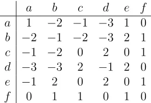
It is because the negative relations are not transitive. Suppose Table 15 is a very small

PMI matrix, and we have the word vectors fora and b. We can see from the matrix that

aand bhave negative relations, and they both have negative relations with cand d. If we

do not remove the negative values in the matrix, the cosine similarity of the worda andb

is positive, which disagrees with the fact that aand b are negatively related. It is mainly

due to the negative values. The third element and the fourth element in both vectors are

negative, if they are multiplied, it would be a large positive value, and the cosine similarity

is a positive value.

Here comes the question: if a is irrelevant to candb is also irrelevant to c, does that

meanaandb are similar? Obviously not. In natural languages, most words are irrelevant

to each other, for example, the words “tiger”, “car” and “next”, the first two words are

both irrelevant to the third word, but they are not related neither. Of course, there are cases

(49)

words are all irrelevant to each other are more common.

It means the negative relations are not transitive, but positive relations are. To remove

the influences of the negative relations, nullifying the negative values is necessary.

4.3 Singular Value Decomposition (SVD)

Though high dimensional word vectors work well, it is always better to have vectors with

lower dimension, because it is faster and easier to generalize. A common way to factorize

the SPMI matrix is to do the Singular Value Decomposition(SVD) [12], which finds the

optimal rankdfactorization according toL2loss.

SVD factorize the m×n matrixM into the product of three matricesUΣVT_{, where}

U andV are unitary matrices, and their shapes arem×mandn×nrespectively. Σis an

m×n diagonal matrix of eigenvalues in decreasing order. To reduce the dimension and keep most information at the same time, we only keep the topd elements in Σ, thus we

have

Md =UdΣdVdT (21)

If we use SVD to factorize the SPMI matrix,Ud·Σdcan be replaced withW, whereW is the word vector matrix, and useVdto represent context vector matrixC, we have

W =UdΣd (22)

C =V_dT (23)

Each row ofW represent the word vector, and the dimension of the vector isd. Each row

ofC is the context vector for each word and the dimension is alsod.

(50)

the quality of word vectors will be better. In this way, we use

W =UdΣαd (24)

C = Σ(1_d−α)V_dT (25)

whereαis usually set to 0.5.

The performance of word vectors from matrix factorization should be similar to that

from Word2vec theoretically, but in our experiment, the SVD vector dose not have much

advantage over Word2vec, and it is not scalable. When the corpus is very large, it is

time-consuming to perform SVD on the co-occurrence matrix, though the matrix is a sparse

(51)

Dynamic Mutual Information (DMI)

To improve the SPPMI, we propose Dynamic Mutual Information, which dynamically

shifts the PMI values according to the variance of ratios, and preserves only the reliable

values. Let r = Fij_ˆ

Fij, andσ 2

r be the variance ofr, the estimation forr is useful only when

its varianceσis within certain range. Applying Chebyshev’s Inequality, we have

P(|r−rˆ| ≥cσ)≤ 1

c2. (26)

This means the probability that the value ofrfalls outside the interval(ˆr−cσ,rˆ+cσ)does not exceed _c12. For example, ifc=

√

2, the probability ofr≤rˆ−√2σorr≥rˆ+√2σis less than 1₂. Also, therˆ= 1, because theFij is expected to be equal toFˆij.

Hence, we derive DMI as follows:

DM Iij =







0, if Fij

b

Fij <

√

2σr+ 1;

logFij b

Fij

−log(√2σr+ 1), otherwise.

(27)

In our DMI, we preserve all the PMIs larger than√2σr+ 1. In the following sections, we will talk about how to get the variance ofr.

5.1 Variance of

r

The variance ofris:

σ_r2 =var Fij

c

Fij

!

= var(Fij)

E(Fb_ij)2

(52)

Letσ2

F be the variance ofFij, we can have

σr =

σF

E(Fbij)

(29)

If we can get the value of σF, then we can calculate σr. However, the distribution of

Fij is pretty complicated, which is shown in Figure 13. The distribution ofFij is similar

to power law distribution whenFˆij is small in a log-log plot, but whenFˆij gets larger, the

distribution ofFij is more like log-normal distribution. It is very difficult to calculateσF

norσr.

However, after examining several data sets, we find that the value ofσrcan be roughly

approximated using the functiony = √a

Fij, as shown in Figure 16. Each dot in Figure 16

represents the variance ofrwhenFˆ = 0−300. There are 7 million word pairs are collected for each plot. For two words in a word pair, they are randomly selected from the corpus,

and the probability of each word being sampled is proportional to its word frequency in

the corpus, which means frequent words are more likely to be selected than rare words and

someFijs can be 0. The window size is 5.