DEVELOPMENT OF A NONLINEAR TIME DOMAIN METHODOLOGY, RESULTS
(PART II)
Robert Spears1, Greg Mertz2, and Justin Coleman3
1
Seismic Engineer, Idaho National Laboratory, Idaho Falls, ID ([email protected]), USA 2
Senior Engineer, CJC and Associates, Los Alamos, NM, ([email protected]), USA 3
Seismic Engineer, Idaho National Laboratory, Idaho Falls, ID ([email protected]), USA ABSTRACT
A complementary paper, “Development of a Nonlinear Time Domain Methodology (Part I),” lays out a methodology to follow when performing nonlinear soil-structure interaction (NLSSI) analysis. This paper presents results from numerical analyses that compare a recently verified and validated version of SASSI with those from a NLSSI code using increasing levels of earthquake ground motion. Comparisons will be presented at multiple locations inside a generic nuclear power plant structure. The generic nuclear power plant (NPP) is placed on a well-studied soil site.
At low levels of ground motion the linear analysis and NLSSI produce similar results with results diverging for higher levels of ground motion. Results show that differences in the spectral accelerations calculated using the equivalent linear and nonlinear methods are observed at significant levels of ground motion shaking. For the NPP analyses, the differences are associated with separation and sliding, which cannot be explicitly represented with equivalent linear analysis.
OVERVIEW
In this paper, Soil Structure Interaction (SSI) results using SASSI (Lysmer et al. 2000) are compared with equivalent linear and nonlinear NLSSI results. SASSI is a linear, frequency domain SSI analysis program. The NLSSI results are developed using the explicit time domain solver in LS-DYNA (LSTC
2013). The LS-DYNA models use a nonlinear soil constitutive model (discussed further in the
MATERIAL PROPERTIES section). Two different approaches are used in the LS-DYNA analyses. The first approach neglects separation and sliding on the soil-structure interface and is referred to as the equivalent linear model. In the second approach, both separation and sliding are allowed on the soil-structure interface and this is referred to as the nonlinear model.
As input for this study, seismic time histories are used that fit 10,000-year rock outcrop Design Basis Earthquake (DBE), 5% damped response spectra specific to the INL site (Payne 2006). The time histories are then scaled to produce 0.5•DBE, 1.0•DBE, 1.5•DBE, 2.0•DBE, and 3.0•DBE input. A representative sample of these results is presented herein.
The results comparisons are performed in two phases. The first phase compares the response of the linear (SASSI) and equivalent linear (LS-DYNA) results to understand differences between the time domain and frequency domain solutions. The second phase studies the changes in response due to separation and sliding on the soil-structure interface.
shear waves. Second, three-dimensional analyses in this SASSI solution are performed as three separate analyses, with one analysis for each component of the seismic time history. The results of these analyses are then combined using square root sum of the squares (SRSS). LS-DYNA performs three-dimensional analyses using all three components of the seismic time histories simultaneously. Third, to translate the structural model from LS-DYNA to SASSI, the model was read into Abaqus/Standard (Dassault Systèmes 2012) and the stiffness and mass matrices were written out from Abaqus/Standard to SASSI. The different element formulations in the two programs are the source of some of the difference in linear analysis results.
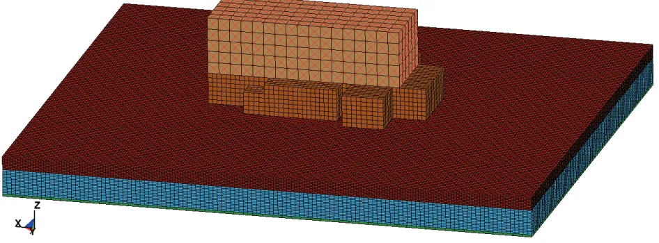
FINITE ELEMENT MODEL
The LS-DYNA SSI model is shown in Figures 1 to 3. The soil mesh consists of upper alluvial soil (UAS), lower alluvial soil (LAS), and basalt. The UAS is 30 feet deep, the LAS is 55 feet deep, and the modelled basalt is 5 feet deep. The horizontal soil dimensions are 1164 x 984 ft (1164 ft in the x-direction).
Figure 1. SSI model.
The elements corresponding to UAS are 2 ft thick, the elements corresponding to LAS are 3.44 ft thick, and the element corresponding to basalt is 5 ft thick. These element thicknesses are selected such that a 40 Hz shear or compressive wave can propagate through the soil profile with at least 10 elements per wave length considering softening in the soil.
The structural model has the enveloping plan dimensions of 479 x 303 ft (479 ft in the x-direction), is embedded 75 feet, and projects 194 feet above the ground surface. For the LS-DYNA explicit solver, the time step is related to the smallest element length divided by the speed of sound through that element. The mesh density in the structure is sized to obtain a stable model time step similar to that of the soil.
Figure 2. Cut-away view of the soil mesh.
Figure 3. Cut-away view of the structural mesh with nodes identified where results are compared.
The boundary conditions for the NLSSI models include non-reflective boundary conditions at the base, free boundary conditions at the top surface, and seismic load time histories applied at the top of the basalt layer. More discussion on the application of these boundary conditions can be found in Coleman et al. (2015).
The nodal positions of the different soil types are not aligned to each other in the soil mesh. The different soil types are tied together using a constraint-based tied contact in LS-DYNA (which constrains the nodes to move together) as opposed to a penalty-based contact (which adds a nonlinear interface spring between nodes). Additional constraints are provided at the lateral boundaries of the soil domain to simulate a horizontally infinite soil continuum. These constraints enable the boundary nodes at each elevation (that form a “ring” around the model) to move together in the horizontal and vertical directions. This allows accurate modelling of the vertical propagation of shear and compressive waves, and provides the required
UAS
LAS
Basalt
Grade
1263
2899
223
1
1 10" !7 1 10" !6 0.00001 0.0001 0.001 0
10 20 30
1 10" !7 1 10" !6 0.00001 0.0001 0.001
0 5 10 15
into the model, rather than transmitted out of the model. With a sufficiently large soil domain, it is assumed that the scattered waves attenuate before reaching the boundary, thus minimizing the internal reflections in the soil domain.
The structure is constrained to the soil for the equivalent linear model runs and is in frictional contact with the soil for the nonlinear model runs. The contact is defined with a penalty contact algorithm and a coefficient of friction of 0.5 which represents the expected friction for sand.
MATERIAL PROPERTIES
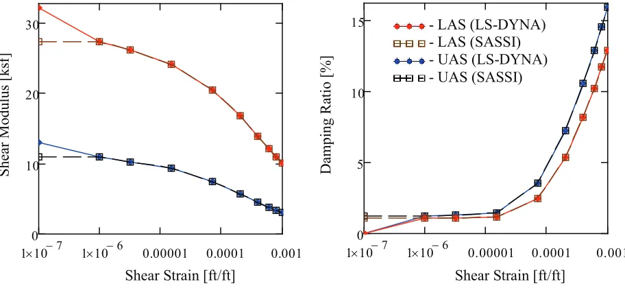
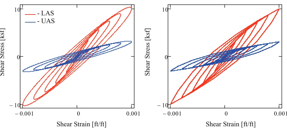
The basalt in the LS-DYNA models is linear and is used as a model boundary where the seismic motion can be input and reflected waves can be allowed to pass out of the model. In the SASSI model, there are multiple layers of basalt over an elastic halfspace of basalt. The UAS and LAS material properties for the SASSI evaluation use the shear modulus and damping properties shown in Figure 4. The equivalent nonlinear material properties used in LS-DYNA for the UAS and LAS are defined using Spears et al. (2015). Figure 5 shows the hysteresis loops that result from the linear material properties (SASSI) and nonlinear material properties (LS-DYNA). The linear material properties hysteresis loop is generated with elastic soil stiffness and frequency independent, viscous damping. The nonlinear material properties hysteresis loop is generated with post yielding shear stress versus shear strain.
For this paper, the linear and nonlinear model material properties (shown in Figure 4) are defined to approximate curve shapes based on Idaho National Laboratory (INL) soils (Payne 2006). The INL soils
are defined for strain values between 10-6 ft/ft and 10-3 ft/ft. In order to approximate a low strain (10-6
ft/ft) damping ratio, the material properties used in LS-DYNA include an added lower strain (10-7 ft/ft)
data point. This is necessary because the nonlinear model energy absorption results from soil plasticity. Consequently, the elastic region (where no energy is absorbed) is made small to allow for energy
absorption at low strain (10-6 ft/ft). Given the scatter in the actual test data, the defined material
properties produce a reasonable representation for the soil.
S
he
ar
M
odu
lus
[ks
f]
D
am
pi
ng R
at
io
[%
]
Shear Strain [ft/ft] Shear Strain [ft/ft]
Figure 4. Shear modulus and damping ratio versus shear strain curves for UAS and for LAS. - LAS (LS-DYNA)
S
he
ar
S
tr
es
s
[ks
f]
S
he
ar
S
tr
es
s
[ks
f]
Shear Strain [ft/ft] Shear Strain [ft/ft]
Figure 5. Hysteresis loops for the linear material properties (left-hand plot) and for the nonlinear material properties (right-hand plot).
The structure is modelled with linear concrete and steel material properties. Damping is represented using 4% Rayleigh damping at frequencies of 5.7 and 15 Hz, which bounds the region of significant structural response.
NONLINEAR SOIL CONSTITUTIVE MODEL
The LS-DYNA hysteretic soil model is used to represent the soil behaviour. This model assumes each element has up to 10 subelements which experience the same strain. Each subelment has a unique stiffness, a unique yield stress, and has an elastic/perfectly plastic behaviour base on a kinematic hardening rule. The response of the subelements is summed together to produce the post yielding shear stress versus shear strain curve that has been defined for the element. Having the constitutive model defined in this manner produces the realistically shaped hysteresis loops shown in Figure 5.
Soil shear stiffness is a function of both shear strain and hydrostatic stress. Consistent with the approach used in SASSI, the current soil modelling is simplified by neglecting changes in shear stiffness due to changes in hydrostatic stress. This simplification allows a direct comparison of the analysis methodology to SASSI results. Future work will investigate the effects of varying hydrostatic stress on response.
RESULTS AND DISCUSSION
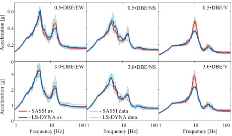
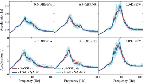
Figures 6 to 9 show the 5% damped acceleration response spectra for the SASSI and equivalent linear LS-DYNA model runs at nodes identified in Figure 3. The spectra show the individual results of five sets of time histories along with the average response. Each of the time histories is fit to the target spectra using the criteria in ASCE 43 (ASCE 2005). Multiple time histories are averaged to smooth out narrow gaps and spikes in the spectral results.
For all of the results, EW (East-West) is the x-direction, NS (North-South) is the y-direction, and V (vertical) is the z-direction in Figures 1 to 3.
0.001
! 0 0.001
10 !
0 10
0.001
! 0 0.001
10 !
0 10 - LAS
A
cc
el
er
at
ion [
g
]
A
cc
el
er
at
ion [
g
]
Frequency [Hz] Frequency [Hz] Frequency [Hz]
Figure 6. Node 1 acceleration response spectra for equivalent linear analyses
A
cc
el
er
at
ion [
g
]
A
cc
el
er
at
ion [
g
]
Frequency [Hz] Frequency [Hz] Frequency [Hz]
Figure 7. Node 2899 acceleration response spectra for equivalent linear analyses. - SASSI av.
- LS-DYNA av.
3.0•DBE/EW 0.5•DBE/EW
3.0•DBE/NS 0.5•DBE/NS
3.0•DBE/V 0.5•DBE/V
- SASSI data - LS-DYNA data. - SASSI av.
- LS-DYNA av.
3.0•DBE/EW 3.0•DBE/NS 3.0•DBE/V
A
cc
el
er
at
ion [
g
]
A
cc
el
er
at
ion [
g
]
Frequency [Hz] Frequency [Hz] Frequency [Hz]
Figure 8. Node 223 acceleration response spectra for equivalent linear analyses.
A
cc
el
er
at
ion [
g
]
A
cc
el
er
at
ion [
g
]
Frequency [Hz] Frequency [Hz] Frequency [Hz]
Figure 9. Node 1263 acceleration response spectra for equivalent linear analyses.
Figures 6 to 9 show good agreement in the East-West and North-South directions especially for the 0.5•DBE. The maximum difference was about 14% and it occurred in the Figure 9, 0.5•DBE/NS plot. The maximum difference in the East-West and North-South directions for the 3.0•DBE about 18% and it occurred in the Figure 9, 3.0•DBE/NS plot. The vertical response for Figures 8 and 9 also showed good
- SASSI av. - LS-DYNA av.
3.0•DBE/EW 0.5•DBE/EW
3.0•DBE/NS 0.5•DBE/NS
3.0•DBE/V 0.5•DBE/V
- SASSI data - LS-DYNA data.
- SASSI av. - LS-DYNA av.
3.0•DBE/EW 0.5•DBE/EW
3.0•DBE/NS 0.5•DBE/NS
3.0•DBE/V 0.5•DBE/V
source of the remainder of this difference.
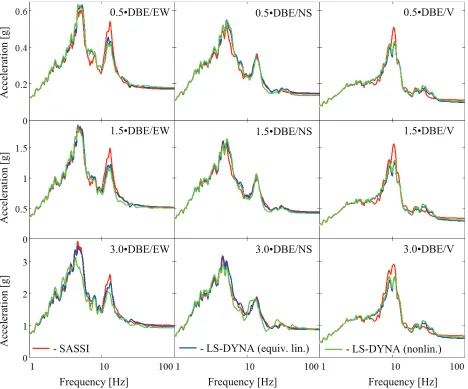
The nonlinear response including the effects of separation and sliding are determined using a single set of time histories developed for the INL site (Payne 2006) and the results are shown in Figures 10 and 11. Results with separation and sliding are labelled nonlinear LS-DYNA. Elastic SASSI and equivalent linear LS-DYNA results, similar to the individual case results above are also presented.
A
cc
el
er
at
ion [
g
]
A
cc
el
er
at
ion [
g
]
A
cc
el
er
at
ion [
g
]
Frequency [Hz] Frequency [Hz] Frequency [Hz]
Figure 10. Node 1 acceleration response spectra with separation and sliding compared to equivalent elastic response.
- SASSI
1.5•DBE/EW 0.5•DBE/EW
3.0•DBE/EW
1.5•DBE/NS 0.5•DBE/NS
3.0•DBE/NS
1.5•DBE/V 0.5•DBE/V
3.0•DBE/V
A
cc
el
er
at
ion [
g
]
A
cc
el
er
at
ion [
g
]
A
cc
el
er
at
ion [
g
]
Frequency [Hz] Frequency [Hz] Frequency [Hz]
Figure 11. Node 2899 acceleration response spectra with separation and sliding compared to equivalent elastic response.
Figures 10 and 11 show somewhat predictable results. Agreement between the SASSI and equivalent linear LS-DYNA are similar to those shown in Figures 6 and 7. As the magnitude of ground motion increases, the difference in response with separation and sliding becomes more apparent. In Figures 10 and 11, the relative EW response decreases at large scale factors compared to the equivalent linear
response with the largest reduction approaching 20%. Similar examples of the nonlinear behaviour
reducing the response can be found in nodes throughout the structure and in all three directions. In the horizontal directions, it appears that the nonlinear behaviour puts an upper limit on the response at a given node. For example, in Figures 10 and 11 both the linear and equivalent linear models show a significant difference in peak horizontal response amplitude at 3.0•DBE compared to the nonlinear models, which show a much less significant difference. This is generally true for all the nodes checked in the structure. Consequently, the most significant reductions due to nonlinear response can be expected where the most significant linear response occurs.
Not all of the results checked in the structure exhibited decreases due to nonlinear response. Some nodes where the structure contacts the soil showed significantly increased response, especially at high frequencies, for the nonlinear models. Some of this increased response can be explained by impact which is a real response that must be considered. Some of the increased response can be explained with contact
- SASSI
- LS-DYNA (equiv. lin.) - LS-DYNA (nonlin.)
1.5•DBE/EW 0.5•DBE/EW
3.0•DBE/EW
1.5•DBE/NS 0.5•DBE/NS
3.0•DBE/NS
1.5•DBE/V 0.5•DBE/V
It is important to note that, for the nodes that were checked in the structure, none of the nodes away from the soil-structure boundary had response increases nearly as significant as those at the soil-structure boundary. This could indicate that the error associated with contact chatter is somewhat local (where increases due to impact and/or associated with excitation of the added contact springs should not be local).
Another option to minimize error associated with contact is to attach the soil to the structure and let the nonlinear soil constitutive model address the contact. This would require that at least the elements touching the structure must be allowed to have a stress versus strain that changes with hydrostatic stress (which is a more accurate way to model soil behaviour). Another benefit of this approach is that rather than having to select a friction factor, the structure plastically shears the soil based on the soil test data.
CONCLUSIONS
NLSSI results are verified by comparing the recently V&V version of SASSI with NLSSI. In general, at low levels of ground motion, the linear analysis and NLSSI produce similar results with results diverging for higher levels of ground motion. Results show that differences in the spectral accelerations calculated using the equivalent linear and nonlinear methods are observed at significant levels of ground motion shaking. For the NPP analyses, the differences are associated with separation and sliding, which cannot be captured explicitly with equivalent linear analysis.
REFERENCES
ASCE (2005), “ASCE/SEI 43-05, Seismic Design Criteria for Structures, Systems, and Components in Nuclear Facilities,” American Society of Civil Engineers, Reston, Virginia, USA.
Coleman, J., Spears, R., and Cohen, M. (2015). “Development of a Nonlinear Time Domain Methodology (Part I).” In: Proceedings of the 23rd SMiRT Conference, Manchester, United Kingdom.
Dassault Systèmes (2012), Abaqus Software, Version 6.12-2, Dassault Systèmes Simulia
Corporation, Providence, RI.
LSTC (2013). “LS-DYNA, Version smp s R7.00,” LS-DYNA Keyword User’s Manual, Volume II,
Livermore Software Technology Corporation, Livermore, CA, USA.
Lysmer, J., Ostadan, F., and Chin, C., (1999), “SASSI2000, User Manual,” Revision 1, A
System for Analysis of Soil-Structure Interaction, University of California, Berkeley, CA.
Payne, S. J. (2006). Data and Calculations for Development of Soil Design Basis Earthquake Parametersat RTC. Research Report, INEEL/EXT-03-00943, Revision 2, INL, Idaho Falls, ID, USA.