Finite Element Analysis of an In Vitro Traumatic Joint Loading Model

ABSTRACT

SHOGE, RICHARD OLUSENI. Finite Element Analysis of an In-vitro Traumatic Joint Loading Model. (Under the direction of Dr. Peter Mente).

Osteoarthritis (OA) is characterized by the degeneration of articular cartilage

resulting in eventual bone on bone contact causing pain and inflammation to musculoskeletal joints. Even though the mechanisms linking joint trauma with post-traumatic OA are poorly understood, joint overloading has been shown to decrease cartilage matrix integrity and is associated with chondrocyte necrosis and apoptosis which are early signs of OA.

An in vitro impact injury model that incorporated tangential loading was developed in our lab using intact porcine patellae to produce quantifiable degradation similar to that seen in early stage osteoarthritis. We carried out two separate sets of in vitro impact experiments: (1) axial impactions: an impact insult normal to the cartilage surface at a high load and relatively fast loading rate and (2) shear impactions: a compressive preload normal to the surface subsequently followed by a tangentially applied displacement generating a shear load. The first impact injury model (axial impaction) had been extensively investigated in the literature and incorporated loads known to cause cartilage damage and cell death. The second model incorporated greater shear forces along with the axial forces and was believed to give a better representation of physiological loading.

A finite element model was created to determine the resulting mechanical stresses and strains in the underlying cartilage tissues. An Ogden hyperelastic constitutive model was used as the input material model for the finite element analysis. Cartilage in our model was broken into three homogeneous tissue zones: surface, mid, and deep and separate

variables examined from the model were location and magnitude of compressive, tensile, and shear stresses and strains.

Intact patellae were maintained in organ culture up to two weeks to investigate the time course of cellular and matrix events post-injury. Cell death and matrix proteoglycan loss were quantified. After validation of the finite element model and collection of histological data, statistical analysis was used to correlate type, location and magnitude of stress and strain with cell death and proteoglycan loss. The overall hypothesis was that shear forces arising from traumatic impact injuries are more detrimental to cartilage matrix and

Finite Element Analysis of an In-vitro Traumatic Joint Loading Model

by

Richard Oluseni Shoge

A dissertation submitted to the Graduate Faculty of North Carolina State University

in partial fulfillment of the requirements for the Degree of

Doctor of Philosophy

Biomedical Engineering

Raleigh, North Carolina 2010

APPROVED BY:

_______________________________ ______________________________

Dr. Peter Mente Dr. Simon Roe

Committee Chair

_______________________________ ______________________________

Dr. Elizabeth Loboa Dr. Mohammed Zikry

ii DEDICATION

iii BIOGRAPHY

Richard Oluseni Shoge was born in New York City, New York in 1982 and raised in Chestertown, Maryland. His parents are Dr. Simeon B. Shoge and Dr. Ruth C. Shoge. He has an older sister, Dr. Ruth Y. Shoge, and two younger siblings: Maryann T. Shoge and Samuel T. Shoge. Richard attended high school at Kent County High School in Worton, Maryland from 1996-2000. He obtained his Bachelor’s of Science in

iv

ACKNOWLEDGEMENTS

v

TABLE OF CONTENTS

List of Tables……….……….………... ix xi 1 1 2 5 5 5 8 10 15 19 22 24 24 24 24 List of Figures……… Chapter 1………...…...

vi

3.1.2. Axial Impact Injury Model……….... 25

27 3.1.3. Shear Impact Injury Model……… 3.2. Development of Cartilage Multilayer Material Model……..…………. 30

3.2.1. Cartilage Hyperelastic Material Model………. 30

3.2.2. Tensile Test Procedure……….. 31

3.2.3. Compression Test Procedure………. 32

3.2.4. Hyperelastic Model Curve Fit……… 33

3.3. Development of the Finite Element Model………... 40

3.3.1. Part and Mesh Definitions………. 41

3.3.2. Material Property Definitions……….... 45

3.3.3. Load and Boundary Conditions Definition……… 46

3.3.4. Validation of Finite Element Model using Pressure Film Analysis……….... 47

3.3.5. Incorporation of Friction……….... 50

3.4. Histology Procedures……….. 51

3.4.1. Patella Culture……… 51

3.4.2. Histology Procedure………... 51

3.5. Statistical Analysis……….. 53

vii

Results……….. 54

4.1. Axial and Shear Impaction Results………... 54

4.2. Cartilage Multilayer Material Model Results………. 60

4.2.1. Tension and Compression Results………. 60

4.2.2. Hyperelastic Strain Energy Function Curve Fit Results………... 63

4.2.3. Axial Impaction Finite Element Model Mesh Validation……….. 65

4.2.4. Axial Impaction Finite Element Model Pressure Film Validation 67 4.3. Axial Impaction Finite Element Model Stress Strain Results………… 70

4.3.1. Multilayered Finite Element Model Strain Results………... 71

4.3.2. Multilayered Finite Element Model Stress Results………... 77

4.3.3. Thickness Parametric Study……….. 94

4.3.4. Axial Finite Element Model with Added Friction………. 99

4.3.5. Comparison of Multilayered Model to Single Layered Model…. 100 4.4. Experimental Axial Impaction Histology Data………... 106

4.5. Correlation of Multilayered Finite Element Model with Histology Data……… 4.6. Shear Impaction Finite Element Stress and Strain Results……… 108 110 Chapter 5……….………... 119

viii

5.1. Experimental Axial and Shear Impaction Results………….…………. 119

5.2. Validity of Multilayered Hyperelastic Model for Cartilage………….... 121

5.2.1. Significance of a Hyperelastic Multilayered Model……….. 121

5.2.2. Comparison Axial Impaction Multilayered Finite Element Model to Single Layered Model ……….……… 124

5.2.3. Axial Impaction Finite Element Model Strain Results….………. 127

5.2.4. Comparison of Finite Element Model Results with Published Literature……….. 129

5.2.5. Pressure Film Validation Results………... 132

5.3. Axial Impaction Finite Element Results- Histology Results Correlation……….. 134

5.4. Shear Impaction Finite Element Model………..……… 136

Chapter 6……… 139

Conclusion………... 139

Literature Cited……….. 141

ix

LIST OF TABLES

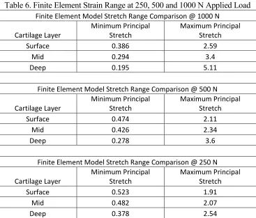
Table 1. Parameter Values for Surface, Mid and Deep Cartilage Layers………….. 65 Table 2. Convergence of Finite Element Model Solution for 2000 N Load……….. 66 Table 3. Axial Impaction Model and Hertz Contact Solution Comparison………... 66 Table 4. Pressure Film – Axial Impaction Finite Element Model Comparison……. 67 Table 5. Experimental-Finite Element Model Stretch Range Comparison for

2000N Load………... 74

Table 6. Finite Element Strain Range at 250, 500, and 1000 N Applied Load……. 77 Table 7. Stress Variables Predicted by 2000 N Load Axial Finite Element Model.. 88 Table 8. Strain Variables Predicted by 2000 N Load Axial Finite Element Model.. 94 Table 9. Effect of Cartilage Thickness on Cartilage Mechanical Behavior……….. 99 Table 10. Effect of Friction Added to Finite Element Model……… 99 Table 11. Stress and Strain Predicted by Multi and Single Layered Axial Finite

Element Model………... 102

Table 12. Correlation Between Percentage Cell Death and Axial Impaction

Multilayered Finite Element Model Stresses and Strains……….. 109 Table 13. Correlation Between Proteoglycan Content and Axial Impaction

x

Table 14. Friction Coefficients and Resulting Reaction Forces Predicted by Shear Impaction Finite Element Model………... 113 Table 15. Peak Stress and Strain Magnitude and Location Predicted by Shear

Impaction Finite Element Model………... 117 Table 16. Stress and Strain Variables Predicted From Axial and Shear Impaction.. 118 Table 17. Axial Impaction Friction Coefficients………..159 Table 18. Shear Impaction Friction Data………..162 Table 19. Pressure Film vs Finite Element Model Comparison at Slow Loading Rate to 500 N Preload for Shear Impaction………..…163 Table 20. Axial Impaction Pressure Film Data……….164 Table 21. Correlation Chart Mean Percentage Cell Death and Stress and Strain

Variables Predicted by Axial Impaction Finite Element Model………....165 Table 22. Correlation Chart Proteoglycan Normalized Intensity and Stress and

xi

LIST .OF FIGURES

Figure 1. Schematic of Rotating Impactor Design………. 26

Figure 2. Impaction Set-up – Mold and Holder………. 26

Figure 3. Shear Impaction Set-up Schematic………. 28

Figure 4. Shear Impaction Set-up – Hydraulic Loading Frames………... 29

Figure 5. Example of Preliminary Stress Stretch Data……….. 35

Figure 6. Total and Reduced Surface Compression and Tension Data – Weight Calculation………. 38

Figure 7. Axial and Shear Impaction Finite Element Model Geometries and Boundary Conditions………. 42

Figure 8. Axial and Shear Impaction Finite Element Model Mesh………... 43

Figure 9. Hertz Contact Analytic Problem Diagram………. 44

Figure 10. Imprint of Pressure Film……….. 49

Figure 11. Cartilage Regions Collected for Histology Collection………. 50

Figure 12. Diagram of Cartilage Sections Taken for Gene Analysis……… 52

Figure 13. Force Data Recorded from Experimental Axial Impaction……….. 55

xii

Impactions………. Figure 16. Scatterplot Showing Average Shear Forces from Axial and Shear Impactions………..

58

59

Figure 17. Shear Impaction Force Curve Variance………...… 61

Figure 18. Uniaxial Tension and Compression Data………. 64

Figure 19. Stress and Stretch with Lines of Best Fit……….. 68

Figure 20. Example of Pressure Film Imprints……….. 70

Figure 21. Plot of Contact Stress Across Imprint Cross Sections……….…. 71

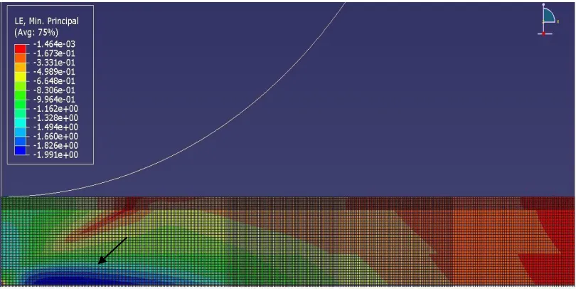
Figure 22. Contour Plot Max Log Strain 2000 N Load……….… 72

Figure 23.Contour Plot Min Principal Log. Strain 2000 N Load……….. 70

Figure 24. Contour Plot Max Principal Log. Strain 250 N Load………... 73

Figure 25. Contour Plot Max. Principal Log Strain 500 N Load………... 75

Figure 26. Contour Plot Max. Principal Log Strain 1000 N Load………. 76

Figure 27. Contour Plot Vertical Stress 2000 N Load……….. 79

Figure 28. Contour Plot Von Mises Stress 2000 N Load……….. 80

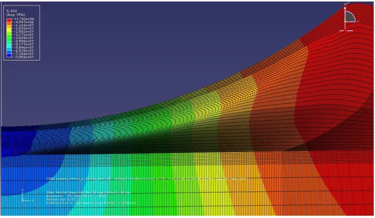
Figure 29. Contour Plot Max. Principal Stress 2000 N Load………..….. 81

Figure 30. Contour Plot Min. Principal Stress 2000 N Load………. 81

Figure 31. Contour Plot Tresca- Maximal Shear Stress 2000 N Load……….. 82

xiii

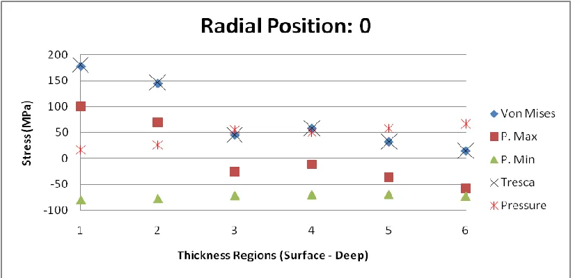
Figure 33. Stress Variables with Respect to Cartilage Depth at Center of Impact… 84 Figure 34. Stress Variables with Respect to Cartilage Depth at Radial Position:

R/2……….. 86

Figure 35. Stress Variables with Respect to Cartilage Depth at Radial Position: R…... 87 Figure 36. Stress Variables with Respect to Cartilage Depth at Radial Position:

2R………... 88

Figure 37. Strain Variables with Respect to Cartilage Depth at Center of Impact… 91 Figure 38. Strain Variables with Respect to Cartilage Depth at Radial Position:

R/2……….. 92

Figure 39. Strain Variables with Respect to Cartilage Depth at Radial Position: R.. 92 Figure 40. Strain Variables with Respect to Cartilage Depth at Radial Position:

2R………... 93

Figure 41. Contour Plot Von Mises Stress Double Thickness Cartilage Model…... 95 Figure 42. Contour Plot Max. Principal Stress Double Thickness Cartilage Model. 96 Figure 43. Contour Plot Min. Principal Stress Double Thickness Cartilage Model.. 96 Figure 44. Contour Plot Tresca Stress Double Thickness Cartilage Model……….. 97 Figure 45. Contour Plot Equivalent Pressure Stress Double Thickness Cartilage

xiv

Figure 46. Contour Plot Max. Principal Log. Strain Double Thickness Cartilage

Model………. 98

Figure 47. Contour Plot Von Mises Stress Single Layered Cartilage Model……… 102 Figure 48. Contour Plot Max. Principal Stress Single Layered Cartilage Model….. 103 Figure 49. Contour Plot Min. Principal Stress Single Layered Cartilage Model….. 103 Figure 50. Contour Plot Tresca Stress Single Layered Cartilage Model…………... 104 Figure 51. Contour Plot Equivalent Pressure Stress Single Layered Cartilage

Model………. 105

Figure 52. Contour Plot Max. Principal Log. Strain Single Layered Cartilage

Model………. 105

Figure 53. Percentage Cell Death With Respect to Cartilage Depth and Radial

Position……….. 106

Figure 54. Proteoglycan Data With Respect to Cartilage Depth and Radial

Position……….. 108

xv

1

Chapter 1

Introduction

Osteoarthritis (OA) is a degenerative disorder affecting the articular joints and is characterized by the breakdown of cartilage covering the joint surface resulting in debilitating pain to those affected [54]. The ability of cartilage to allow smooth and painless transmission of joint forces is highly dependent on the condition of the cartilage tissue which in turn is dependent on the health of the cellular components. The final stages of osteoarthritis have been well documented in the literature but unfortunately, the pathways that initiate cartilage degeneration and osteoarthritis are still unknown. The best approach to finding a solution to osteoarthritis is investigating the mechanisms responsible for its progression over time.

Traumatic joint injuries have been shown to be a predisposing factor for

2

In this study, we directly impacted porcine patellar cartilage using hydraulic loading frames in order to create traumatic joint injury. Two experimental set-ups were used to create injury: (i) an axial impaction model which consisted of a predominantly compressive load and (ii) a shear impaction that incorporated compressive and

tangential loading to the articular surface. After impaction, impacted patellae were maintained in culture for up to two weeks to follow the progression of degenerative changes. Numerical models of the axial and shear impaction were created using the finite element analysis software, ABAQUS, which incorporated a hyperelastic material model for cartilage, to determine the stress-strain distribution within the cartilage and bone layers. Correlations were then made between the stresses and strains within cartilage predicted from the axial finite element model and the histology data to determine possible mechanical causes of cartilage tissue damage.

Specific Aims

3

surface. From this model, areas of high shear, compressive and tensile stress predicted from the model will be correlated to regions of tissue damage. Hypothesis #1: A hyperelastic material model will effectively describe cartilage nonlinear large strain behavior in compression and tension. The predicted contact stresses on the cartilage surface from our finite element model will match contact stresses determined using pressure film analysis. Hypothesis: #2: The use of three distinct isotropic

homogeneous materials models representative of the three cartilage layers incorporated into the finite element model will produce stress distribution within the cartilage that better correlates with observed tissue damage than single layer models. With the multilayered model compared to single layered models, stress concentrations are predicted at the interfaces between tissue zones because of the difference in properties. The region with the largest difference in tissue properties, the calcified cartilage-deep cartilage interface, should coincide best with the area shown to have the most tissue damage from histology studies.

4

and strain results calculated by the shear impaction finite element model will be used to predict where tissue damage is likely to occur.

The general hypothesis underlying these specific aims is that following an injury chondrocyte viability and integrity of the cartilage matrix depend critically on the type and magnitude of mechanical stress the tissue undergoes and it is suspected that shear stress is the main culprit for inducing chondrocyte death. Both mechanical loads: axial and shear, must be incorporated in order to realistically simulate an impact injury to articular cartilage. However, most previous impact injury studies have primarily focused on the response of articular cartilage to axial loading which means the true extent of damage to cartilage may be underestimated.

This injury model has clinical relevance because it can potentially allow us to identify how and the extent to which cells and matrix components are affected by detrimental forces resulting from traumatic injuries during a time period where therapeutic treatment of the injury may be the most beneficial. Identifying and

5

Chapter 2

Background

2.1. Cartilage Structure and Function

Articular cartilage is an amazing and complex structure. It is the soft connective tissue that covers the bony surface of articulating joints and is responsible for the transmission of joint forces and joint lubrication [46]. Most importantly, it contributes to the low friction environment within the joint and allows for pain free motion. These essential qualities result from the unique structure of the tissue which includes a solid phase, comprised primarily of type II collagen and proteoglycans, and a fluid phase. Type II collagen fibers are long fibrous structural proteins that give cartilage its tensile strength [46]. Proteoglycans (PG) are a type of glycoprotein which consists of a core protein and highly negatively charged glycosaminoglycan chains. This negative charge density is what gives cartilage its superior compressive strength due to the repulsion of like charges and the attraction of water. The pull of water into the tissue creates a swelling pressure which pre-tenses the collagen fibers and limits fluid flow within the porous matrix. Proteoglycans form larger aggregates called aggrecan, and together with collagen type II, contribute to most of the dry weight of cartilage.

6

filled with fluid [46]. Articular cartilage contains about 70% water by weight, and when under stress, this fluid flows throughout the matrix creating a drag force as it passes through, thus giving cartilage its viscous characteristics. As compression increases, the fluid can become trapped and this effect contributes to the stiffening behavior cartilage exhibits at fast loading rates [46]. This stiffening behavior also contributes to its exceptional compressive strength. In effect, the material properties of cartilage depend on the state of the fluid phase [71].

7

be stretched, indicating the direction of the fibers. The chondrocytes in this layer tend to be elongated and lie parallel to the joint surface [66].

The middle zone (40-60% of cartilage height) has the highest concentration of proteoglycans. Collagen fibers have larger diameters [70,71,72,73,74] and their orientations are more random although studies done by Clark [31] have suggested that this randomness may be caused by mechanical damage during specimen preparation. Chondrocytes tend to have a spherical shape in this region. The deep zone (30% of tissue height) also has a large PG content but lower water content than the superficial and mid region. Within the deep zone, collagen fibers are anchored in the calcified cartilage and run perpendicular to the cartilage-bone interface. The calcified cartilage region is the transition zone from cartilage to bone. Hydroxyapatite, the same inorganic constituent found in bone, is found in this zone and gives this tissue its rigidity. A demarcation exists between the deep cartilage and calcified cartilage zone and is referred to as the tidemark. As a result of this structural heterogeneity within the cartilage matrix, tissue material properties also vary with respect to depth within the matrix.

8

the synovial fluid provides nutrients and removal of wastes duties for the cartilage tissue through diffusion. One very important quality the synovial fluid has is contributing to the nearly frictionless motion between contacting articular surfaces [46].

2.2. Clinical Relevance:

Arthritis is one of the most common medical problems and the number one cause of disability in America [27]. There are different kinds, but the most common is osteoarthritis [104]. Based on a survey done in 2001 through the Behavioral Risk Factor Surveillance System, the disease affected about 69.9 million adults in the US [17] (about 10% of the population over the age of 60). The cost to the US healthcare industry is more than $60 billion per year [27]. Symptoms include persistent joint pain and stiffness; radiographs show evidence of articular cartilage loss, bone spurs,

increased subchondral bone density and cysts on the bone surface [27]. The smooth cartilage surface becomes rough, and fibrillation and softening occur

(chrondromalacia) in areas of greatest pressure and joint movement [109].

9

reduces the load-bearing capabilities of the tissue with potential for further destruction of the tissue [74]. Histologic features include cartilage clefts, loss of the cartilage layers, cellular necrosis, chondrocyte cloning, and a duplication of the tidemark. Complicating matters is the fact that cartilage has a limited ability to repair itself following disease or injury. Thus when damaged, the pre-existing composition, structure, and material properties are never completely restored and continued loading of damaged cartilage leads to progressive loss of extracellular matrix. The final stages of osteoarthritis have been well documented in the literature

[18,19,20,25,31,34,38,39,40,42,43,68,69]; and it is during this end stage that treatment is generally sought. Clinically, however, despite the developments of surgical

interventions that can restore joint stability and function, these procedures do not offer long term solutions [56]. This underscores the importance of finding early solutions to cartilage degeneration when the events may be reversible.

The causes of OA are multi-factorial; various factors such as obesity, injury, age, and genetics have been identified to initiate the disease. However, the cellular mechanotransduction pathways and molecular mechanisms that initiate the

10

injury is a discrete event. Patients who have sustained a traumatic joint injury have an increased risk of OA in that joint [54]. Therefore the use of impact injury models can give us a better understanding of the general pathogenesis of OA.

2.3. In vivo Osteoarthritic Models:

Studying the early degeneration of cartilage in humans is difficult to conduct, thus animal models provide a practical tool to study the disease process. These models have included procedures that disrupt the normal physiology of the joint

11

Besides indirect trauma to the articular surface, short duration high pressure impact loads are also known to cause detrimental effects to the cartilage matrix and the cells underneath [5,90,95,96,97,123]. Popular methods used to simulate traumatic joint injuries included blunt impacts to the cartilage surface using either drop towers or servo-hydraulic machines. This experimental model is advantageous because it is simple, repeatable, allows testing of intact cartilage samples and provides an ideal approximation of the sharpness and speed of a traumatic joint injury. These impact models have included single and multiple in vivo impactions

[39,44,45,90,95,96,97,107,108,141] and single and multiple in vitro impactions with cartilage explants [19,20,38,40,44,45,68,69,78,84,86,124,147]. From these models, documentation of several types of degeneration commonly found in early and late stage osteoarthritis within the extracellular matrix such as proteoglycan loss, cell cloning, and crack development on the surface and in the calcified cartilage region were made [6,20,39,59,69,127, 126,141,140]. For instance, Borelli et al. [20] observed a

12

in tissue hydration and a decrease in precursors for leucine and glycosaminoglycans (GAGs), components important in chondrocyte metabolism, with increasing impact energy. Using an in vivo model, Haut et al. [59] recorded a high frequency of surface cracks and softening of the cartilage after impaction of rabbit knees. Ewers et al. [45] impacted cartilage plugs to 158, 633, and 1267 N and observed an increase in surface lesions where cell death primarily occurred.

In vivo models have contributed substantial information about the mechanical factors that contribute to the OA process. However, they do not allow the mechanical insult to the tissue to be quantified. In joint instability models the actual joint loading across the joint cannot be accurately measured. This problem may develop from the inability to completely define the contributions from all anatomical components such as ligaments and tendons and mathematically describe the motion of the articulating surfaces. In vitro models, using systems capable of controlling load and displacement, even though sacrificing the exact anatomical environment, offer better repeatability, and a more accurate analysis of the mechanical factors that are applied to the tissues so the specific causes of degenerative mechanisms can be studied.

The majority of studies have focused only on axial loading of tissue

13

Tangential or shear forces are often ignored because of the low coefficient of friction between contacting articular surfaces during low impact loads. The coefficient of static friction for synovial joints has been measured as less than .01 [46] which is a 100times lower than the smoothest artificial materials. However, high normal contact forces resulting from traumatic injuries can cause frictional forces that are not insignificant for the tissue to resist [3] and these forces have been shown to influence matrix integrity and chondrocyte metabolism. Research has linked large shear strains and stresses to fissures on the articular surface [15,42,43]. In order to understand how chondrocytes respond to shear stress, investigators have used fluid flow to induce shear upon isolated monolayered chondrocytes [135]. Smith et al. used an in vitro study where shear was applied using a cone viscometer at stress levels of 0.16, 0.41, 0.82, and 1.64 Pa [135]. They observed an upregulation of interleukin-6, an immunoregulatory cytokine found upregulated in osteoarthritic tissues, and nitric oxide, which is also upregulated in OA tissue. However, despite degrading conditions, they also observed an increase in glycosaminoglycan synthesis compared to unstimulated controls.

The fluid induced shear studies show that fluid flow can significantly affect chondrocyte metabolism, however, under tangential loads applied to the intact cartilage matrix, the stiffness is resisted by intra and inter-molecular cross-links between

14

integral part of the mechanical properties of cartilage under compressive loading, there is no intratissue fluid flow under shear loading because the specimen volume is

preserved as the matrix deforms [151]. Researchers have had success promoting cartilage matrix synthesis from application of dynamic shear directly to the cartilage surface. Using an in vitro model, Grodzinsky et al. applied between 1-3% dynamic shear strain to the cartilage surface at frequencies of .1-1.0 Hz up to 24 hours. This strain range was believed to be in the range of physiological tissue loading [50]. They reported that dynamic shear forces applied at low constant amplitudes can increase the rate of matrix synthesis in cartilage explants and appear to favor synthesis of collagen over proteoglycans [50]. Waldman et al., carried this same dynamic shear study for longer periods of time, up to a week, and found that collagen and proteoglycan synthesis was increased by approximately the same amount when subjected to intermittent shear loading [144]. All in all, Grodzinsky et al. [50,56] and other

researchers has shown a positive effect on cartilage metabolism caused by simple shear loading of articular cartilage, but at low strains and frequencies.

15

where large compressive and shear forces are expected, have not included the effect of shear loading on cartilage integrity. Instead, impact injury models have shown

detrimental effects on chondrocyte gene expression and viability when subjected to large axial strains and rapid displacement rates that take place in traumatic injuries. The specific role shear loading has upon the maintenance of the cartilage matrix, how it affects chondrocyte gene expression and viability, and how it compares to hydrostatic loading of the matrix and chondrocytes would need to be determined to truly

understand the initiation of specific mechanical pathways that cause cartilage degeneration.

2.4. Analytic Models of Articular Cartilage Behavior:

16

models [65,6,88,64,102], triphasic models [76,77], and non-linear models

[64,80,81,64,90,95]. The first models were derived from linear elastic theory where cartilage was treated as a homogenous isotropic material. Hirsch [132] applied the Hertz solution for contacting elastic bodies to measure the Young’s modulus of articular cartilage. Sokoloff et al. [136], Kempson et al. [71], and Hayes et al. [60] modeled cartilage as an elastic layer and determined the material properties such as the elastic and shear modulus using a variety of tests such as indentation, compression and torsion tests. These linear elastic models offer the advantage of describing the

mechanical response of materials with only two parameters: the Young’s or shear modulus and Poisson’s ratio. Due to the time dependent response of the tissue, usually two values for the elastic modulus were determined: the instantaneous and relaxed or equilibrium modulus [60,71,136]. Again, these elastic models only provide information on the instantaneous or equilibrium time-independent behavior of cartilage over a small strain range. These models are limited because of their inability to describe the

transient response of the material such as creep and stress relaxation as well as non-linearity and large strain behavior usually exhibited by cartilage.

17

Maxwell models, to simulate elastic and fluid characteristics. Hayes et al., [60] used a Kelvin system of dashpots and springs to represent cartilage’s creep compliance. Parson et al. [116] determined the unrelaxed and relaxed shear modulus of cartilage from indentation tests. Hayes and Bodine [61] in 1978 measured the viscoelastic complex shear modulus for bovine articular cartilage using a sinusoidal shear

generator. Using these methods, future investigators were able to determine the time dependent properties of cartilage; however, these constitutive models neglected to describe the interstitial fluid flow seen in cartilage.

The free fluid movement in and out of the cartilage body is restrained by the proteoglycans and the collagen network, thus fluid flow is dependent on the

permeability of the cartilage matrix. Mow et al. [102] proposed a biphasic model which was based on mixture theory and accounts for fluid flow through the tissue. It models cartilage as two distinct phases: a porous, linear elastic solid phase which is permeable to fluid flow and an incompressible fluid phase [103]. Interaction between the solid and liquid phases comes from the frictional drag caused by the relative movement of the fluid phase through the solid phase during deformation. Fluid flow and solid

18

the material response using linear material constants: permeability, k, aggregate modulus, HA, Poisson’s ratio, ν, and solid phase volume fraction,

α

constants are obtained from curve fits of experimental creep and stress relaxation data. This model has been expanded over the years to incorporate viscoelasticity of the solid phase components (proteoglycans and the collagen fibers) [101,102,152]. Inclusion of these intrinsic viscoelastic properties have come to make up the biphasic

19

and the constitutive relationship was curve fit to tensile and compression stress strain data. Another model that incorporates the phenomenological response of biological tissue and has shown favorable results in describing soft biological tissue mechanical behavior is the hyperelastic model [14,50,64]. Ateshian et al. [14] have shown the ability of the hyperelastic function to fit transient finite deformation curves of cartilage and Garcia et al. [50] have demonstrated the ability of a hyperelastic model developed by Holmes and Mow [64] to describe the nonlinear and viscous effects of the solid phase using finite element software.

2.5. Numerical Models of Cartilage Deformation:

20

injuries. Eberhardt et al. [42,43] used an analytic multi-layered Hertzian contact model to model the canine patellae impactions of Thompson et al. [140]. The rabbit patellae impactions of Haut and coworkers [59] were modeled using a 2-dimensional quasi-static finite element model [82]. Quasi-quasi-static stress analysis is used to analyze linear or nonlinear problems with time-dependent material response (creep, swelling,

viscoelasticity, and two-layer viscoplasticity) when inertia effects can be neglected [1]. Anderson et al. [5,6] created a dynamic 2-dimensional plane strain finite element model to model the rabbit knee impactions of Radin et al. [125,126]. They, however, did not find any significant differences in stress distribution over the quasi-static solution [6], suggesting that a quasi-static solution is sufficient for the calculation of the prevailing tissue stresses. Moreover, the potential error associated with this quasi-static assumption was investigated using a discontinuous-medium model by Li et al. and they showed peak load to be altered by at most ± 6 percent [15,80].

Most of these models assumed linear elastic material properties for both the cartilage and bony layers, which is acceptable for high speed loads, but, as stated earlier these parameters do not account for large deformation. Mente et al.

21

are more recent models by Wilson et al. [147,148] and Li et al [81] that expand upon poroviscoelastic theory and combine fiber reinforcement into the model to account for nonlinearity. With these models the solid stress is represented by the sum of the matrix and fibril stresses. As strain increases, the fiber properties account for the stiffening of the tissue. Since the fiber direction has to be accounted for, these fiber reinforced finite element models also characterize the anisotropy of the matrix.

There are a couple shortcomings to these models. For one, any relative tangential motion between the two impacting joints or load contributions from the ligaments, muscles, and other joint structures was ignored. Eberhardt et al. [43]

examined the effects of friction using their layered Hertzian contact model but found it added little to the tensile stresses that they assumed were necessary for crack

22

computationally expensive but these differences may be very significant in explaining damage differences observed in different layers of the tissue [147].

Lastly, the incorporation of viscoelastic behavior may not be necessary for modeling high speed impactions. Oloyede et al. and others have shown that the viscoelastic behavior can be simplified to an elastic model at high loading rates

[5,42,43,82,112,113]. Due to cartilage stiffening and the short loading time during high speed impacts, fluid flow is constrained making it an insignificant factor in cartilage deformation [6,43]. Moreover, as stated earlier fluid flow plays less of a role in cartilage’s shear mechanical properties.

2.6 Purpose:

23

tangential loading. Our multilayered hyperelastic material model was validated by comparing peak stress and contact area predicted from our model with measurements from pressure film tests of the axial impactions.

24

Chapter 3

Experimental Procedure

3.1. Experimental Impact Injury Model 3.1.1. Tissue Preparation

Intact porcine knee joints were collected from a local slaughterhouse. Porcine tissue was chosen because of its abundance in North Carolina and the ability to obtain fresh tissue within two hours of slaughter. Tissue was obtained from retired sows of unknown age with a minimum weight of approximately 180 kg. After the knee was wiped down with betadine and alcohol, the patella was removed sterilely from the knee joint capsule and kept moist throughout the impaction procedure by periodic

application of sterile phosphate buffered saline (PBS) containing antibiotics. Only patellar cartilage with no visible pre-existing defects to the cartilage surface was used. All equipment that came into contact with the patellae such as dissection and culture tools were autoclaved for 60 minutes at 121oC.

25 3.1.2. Axial Impaction Injury Model:

The impacting surface was a 10mm long, 10mm diameter stainless steel

cylindrical impactor (Figure 1, Figure 2e). The impactor was oriented with the cylinder axis perpendicular to the loading direction and running along the medial-lateral axis of the patellae (Figure 2e). The steel impactor was specially designed to rotate along its radial axis, allowing the impactor surface to adapt to various curvatures while applying a relatively uniform load along its long axis (Figure 1). Spherically bottomed

polymethyl methacrylate (PMMA) molds (Figure 2a) were used to encapsulate the patellar bone, which was then placed in a well fixture (Figure 2b) underneath the impactor. Stainless steel bolts were used to align and secure the PMMA mold within the mating spherical cavity that allowed the patellae to be aligned visually so that the cartilage surface target area was perpendicular to the impactor and to prevent

26

B

Figure 1. Schematic of rotating impactor design. The diagram on the left shows that the cylindrical impactor rotates with respect to the r axis. The axial direction is the vertical direction and is the direction the actuator travels towards the cartilage surface. The longitudinal (l) and radial (r) directions are perpendicular to the axial direction and are parallel to the cartilage surface. The diagram on the right shows how the impactor is oriented when it makes contact with the cartilage surface. The axial and radial directions

Targeted axial loads of 2000 N were applied at a displacement rate of 25 mm/s. A three degree of freedom piezoelectric load cell was used to measure forces in the axial, radial and longitudinal direction. The axial direction is normal to the cartilage

C B

A D E

27

surface. The radial and longitudinal directions are orthogonal to the axial direction, with the longitudinal direction corresponding to the 10 mm length of the impactor (Figure 1). Force and displacement data was recorded and saved using LabView (National Instruments, Austin, TX, USA) software. Tissue marking dye was used to create marks on the cartilage surface at each end of the impactor to provide reference markers to identify the impaction region.

3.1.3. Shear Impaction Injury Model:

For the shear impaction design, patellae were obtained using the same

procedures as the axial impactions. For the shear impaction set-up, the x-y positioning jig (Figure 2b), in which the patella is secured, is bolted to a moving platform that can translate in one direction (Figure 3). The moveable platform is attached via pulley system to a second hydraulic loading frame (Instron 8501, Instron Corporation,

Canton, MA) (Figure 4). This second loading frame pulls the moving platform and x-y positioning jig at a specific speed. With this set-up, the patella is subjected to a

28

Figure 3. Axial applied load for shear impaction. A. X-Y positioning jig with secured patella in PMMA mold. B. Schematic of X-Y jig secured to moving platform underneath. After the 500 N load is applied, the impactor is kept stationary as the tangential

displacement takes place. For the angle shown above, the patella would be translated into the plane of the picture by the Instron second hydraulic loading frame (Figure 4).

Axial applied load

29

Figure 4. Shear impaction set-up. A. The MTS loading frame on the right applies a ramped preload of 500N then remains stationary as the Instron loading frame on the left translates the moving platform 5 mm. The Instron and MTS machines are connected together with grip arms. B. A stop bar is bolted to the base of the MTS platform and ensures that the base translates the set distance.

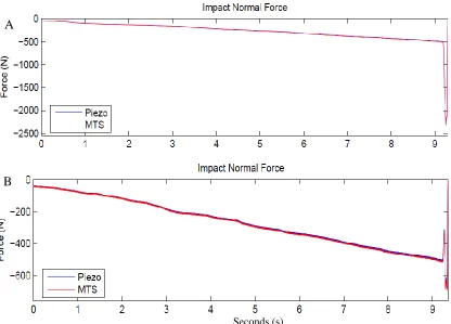
An axial preload of 500 N at a displacement rate of .05 mm/s was applied to the cartilage surface using the MTS hydraulic loading frame and after the peak load of 500 N was reached, the displacement of the MTS actuator was held constant while the moveable platform was displaced tangentially underneath the impactor 5 mm at a rate of 200 mm/s in the radial direction creating the shear load. The purpose of shear impactions was to determine how dynamic shear influences initial damage and

subsequent chondrocyte response. From preliminary work in our lab, axial peak loads of 500 N at displacement rates of .05 mm/s produced minimal macroscopic damage to the cartilage surface. A tangential displacement rate of 200 mm/s has been observed from previous work in our lab to create normal forces (axial-direction) that can reach the 2000N axial force recorded from the axial impactions. This may be due to the

30

irregular topography of the cartilage surface or because the cartilage surface was at an angle and the impactor had to translate uphill.

3.2. Development of Cartilage Multilayer Material Model 3.2.1. Cartilage Hyperelastic Material Model:

In order to understand the mechanical behavior of cartilage, a constitutive stress-strain material model was developed. A hyperelastic material model was selected because of its ability to describe nonlinear compressive and tensile behavior at large strains and because of its success in modeling the elastic response of biological tissues [23,57,105,106,111,144]. Hyperelastic materials are described in terms of a strain energy potential, U, which defines the strain energy stored in the material per unit of reference volume (volume in the initial configuration) as a function of the strain at that point in the material [1]. In order to develop the constitutive material model of articular cartilage, the tensile and compressive stress-stretch responses were determined.

31

cartilage were chosen to create a more accurate model of the disparity in material properties with depth from the cartilage surface.

3.2.2. Tensile Test procedures:

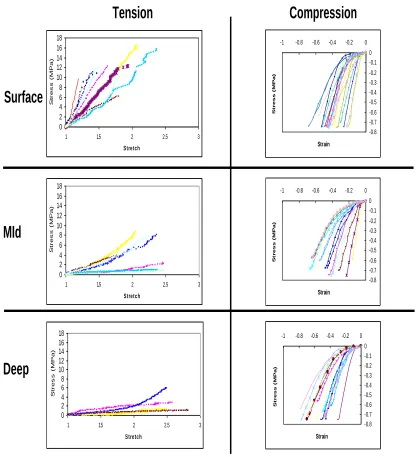
M. Prasath conducted the tension and compression work for his master’s thesis [120]. Rectangular sections, 15 X 4 mm, of cartilage attached to the subchrondal bone were cut from the most flat and smooth portion of the patella. Thin strips 120 μm thick were further cut from the tissue in the three zones for tensile testing. Classification of the sections into the different zones was done by taking the first 10% of the total number of sections in each block to be in the surface zone, the next 60% was regarded as the mid-zone and the last 30% were regarded as the deep zone. Rectangular tensile strips of cartilage measuring 15mm by 2mm were then obtained from each section. Each tensile strip was marked with evenly spaced dots 2 mm apart using tissue marking dye (Polysciences, Inc., PA) which served to mark the initial gage length. Testing was carried out at a displacement rate of 25 mm/sec to simulate the loading rate during our experimental impaction. A total of 30 specimens were obtained; eleven from the surface zones, eleven from the mid zones and eight from the deep zones. All specimens were oriented parallel to the split line axis and loaded to failure.

32

Motionscope, San Diego, CA) at 250 fps. The camera was used to obtain high speed images of the displacement of the ink dots on the specimen. Obtaining deformation data using this procedure eliminated errors due to slippage at the grips and machine and holder compliance. The difference in positions of the dots in the first image was taken as the initial length. Stress (

σ

λ

λ

0

L L

and

σ

where Lis the current distance between the dots per frame, L₀is

the distance between the dots in the first frame, F is the applied force and A is the original cross sectional area of the specimen.

3.2.3. Compression Test Procedures:

33

cartilage compression specimens, were punched out, placed in saline and frozen at -80 C to await testing.

Individual specimen thickness were recorded by taking the initial position of the top plate in contact with the bottom plate and then placing in the specimen and recording the position of the top plate in contact with the specimen at a tare load of 2 g (0.02 N). The difference between the two positions of the actuator gave the thickness of the specimen. A total of 23 specimens from the surface zone, 23 from the mid zone and 21 from the deep zone were tested in compression. Compressive stretch was calculated by dividing the current thickness by the initial thickness L0. Compressive stress

calculations,

σ

A

F _{where F is the applied force and A is the cross-sectional area,}

were carried out assuming that the specimens were perfectly circular. The cross-sectional area was calculated using the formula for calculating the area of a circle,

4

2 D



where D, the initial diameter was taken to be 2.75 mm for all specimens.

3.2.4. Hyperelastic Model Curve Fit:

34

Ogden function. An Ogden model was chosen over other hyperelastic functions because of its flexibility in fitting multiple experimental test data with minimal

coefficients. The coefficients derived from the Ogden hyperelastic model [1,110] have shown favorable results when used to create a curve that fits tensile and compression data from cartilage (Figure 5) particularly over large deformations [90]. The Ogden hyperelastic model, as well as the other available functions in finite element programs, was described in terms of a strain energy potential, U, which is a function of deviatoric (shear) and volumetric components of the strain tensor. The deviatoric response of the material relates to deformation where a change in shape occurs without a change in volume, while the volumetric term relates to a change in volume without deformation. The general form of the Ogden formulation [1] is,





N i i N i i i

_J

D

U

1 3

2 1 1

2

(

1

)

1

3

2

















_

_







where the terms in the first summation make up the deviatoric component and the terms in the second summation make up the volumetric component of the strain energy potential. Within the strain energy function (U)

λ

, λ

λ

35 approximated by curve fitting

the function to experimental stress-stretch data. D and Jel are the compressibility

coefficient and elastic-volume ratio respectively.

An assumption made for the cartilage material model is that it is

incompressible. This means

there is no change in volume when the material deforms corresponding to a Poisson’s ratio of 0.5. Cartilage is assumed to be incompressible because at high loading rates, the interstitial fluid which accounts for most cartilage deformation and viscoelasticity is held in place and is unable to move. Studies have shown Poisson’s ratio of cartilage to be greater than 0.4 at low strain rates [61] and increasing the rate significantly

stiffened the cartilage [112,113,114] during uniaxial testing. Wong et al., [149] verified the assumption of cartilage incompressibility and determined a Poisson’s ratio of .49 in unconfined compression at fast loading rates. Therefore, with this incompressible

Figure 5.Example of preliminary experimental stress stretch data for hyperelastic material fit. The

36

assumption, the volumetric terms of the Ogden strain energy function were set to zero. This reduced the Ogden formulation to:





2 3 2 1 2    



U   

 

Equation 2

Stress was calculated using the principle of virtual work by the equation .





U  Equation 3

For uniaxial tension and compression, which assumes pure homogeneous deformation, the principle stretches,











1



 

2  3  1 for an incompressible material. Therefore using the principle of virtual

work, the equation for stress simplified to:



2 _ 













37 2 1

1



















w

E





w, is the weighted parameter, n is the number of data points, test

i



from the test data and th

i



using the principle of virtual work. A weighted least squares algorithm was chosen because of the larger data variability in tension than in compression. Weights were calculated from the variance in stress using the following equation (Equation 6):

vi i

w



1

 Equation 6

where σvi is the variance in stress. In order to calculate the variance, the compression

38

Total Surface Data

-2.0E+06 0.0E+00 2.0E+06 4.0E+06 6.0E+06 8.0E+06 1.0E+07 1.2E+07 1.4E+07 1.6E+07 1.8E+07

0 0.5 1 1.5 2 2.5

Stretch S tr e s s

Reduced Surface Data

-2.0E+06 0.0E+00 2.0E+06 4.0E+06 6.0E+06 8.0E+06 1.0E+07 1.2E+07 1.4E+07 1.6E+07 1.8E+07

0.0 0.5 1.0 1.5 2.0 2.5

Stretch S tr e s s

Figure 6. Total and reduced surface compression and tension data used to determine curve fit. The total surface data is the complete data set from tensile and compression tests. The reduced surface data plot contains the averages of every three stretch and stress value. The standard deviation was calculated from each group of three and this was used to calculate the weights for the nonlinear least squares curve fit algorithm.

The average stress values were then plugged into the following equation to determine the stress variances:



 3 ( )

i i vi

n

x 

 Equation 7

where xi is the stress,  is the average stress, and n is the number of stress values in

each group. A program was created in FORTRAN (Compaq Visual FORTRAN 6) that created the reduced surface, mid, and deep data sets and calculated the weights using equations 6-7.

39

ABAQUS and results in a total of 12 material constants). The larger the value of N, the more variables the algorithm could adjust to achieve a better fit of the data.

An important consideration in judging the quality of the fit to experimental data is the concept of material or Drucker stability. The Drucker stability condition for an incompressible material requires that the change in the stress,d , following from any infinitesimal change in the logarithmic strain, d , satisfies the inequality:

0 3 3 2 2 1

1        

 d d d d d

d for isotropic elastic materials. This requires the tangential material stiffness to be positive-definite [1]. We satisfied this requirement by requiring the hyperelastic function be monotonically increasing for every value of stretch within the stretch range of the material. This constraint is exemplified by the following equation: 0 ) 1 2 ( ) 1 ( 2 1 1 2 1               



To impose this restriction on the curve fitting algorithm, the nonlinear

40

and the constraint (Equation 8) was imposed at intervals of .01 ranging from .2 to 2.5 (domain of stretch values). One of the major drawbacks to using hyperelastic models was the fact that the accuracy of the model cannot be compared and verified with a known solution because there were no established hyperelastic materials with well defined material properties with which to test the procedure.

3.3. Development of the Finite Element Model:

41 3.3.1. Part and Mesh Definitions

The finite element model consisted of two parts: an analytically rigid impactor and a deformable porcine patella. A 2-D plane strain model of the parts was used to represent a cross section in the middle of the impactor. Since plane strain was used, out of plane strain was considered zero. This was opposed to using plane stress 2-D

analysis because out-of-plane dimensions were not significantly smaller than in-plane dimensions, thus assuming out-of-plane stress to be zero was inappropriate. To test the plane strain assumption, a 3-D model of the axial impaction was done with equivalent part, interface, mesh, and boundary condition definitions as the 2-D model. The stress and strain distribution from the middle cross section of the impactor in the 3-D model was compared to the 2-D results.

42

Figure 7. Axial (left) and shear (right) impaction part and boundary condition definitions. The impactor and cartilage on the left were modeled with a symmetrical axis at the center of impaction. The shear impaction was modeled fully. The tissue layers were created by partitioning the initial block. Boundary conditions were applied to the left and bottom of the axial impaction model. Boundary conditions were applied to the bottom and both sides in the shear impaction model.

43

accuracy of the solution [1]. The cartilage elements were modeled as incompressible hybrid elements which mean a very small change in displacement produces large changes in hydrostatic pressure within the element. Hybrid elements do this by

employing a Lagrange multiplier to add a hydrostatic term where a hydrostatic pressure can be added without changing the displacements [1].

44

include the cartilage layers and the top of the bone. 8 and 4 noded quadrilateral plane strain elements were used for cartilage and bone analysis respectively.

Element size and shape were dictated by how well the solution algorithm could handle large deformation. Consideration was taken into how the elements looked after load was applied to ensure completion of the model solution. The larger aspect ratio elements were oriented so that when compressed element distortion was reduced thus preventing divergence of the equilibrium solution. In the stiffer tissues farther away from the impaction zone such as the subchondral and trabecular bone, the number of elements was decreased since less deformation occurred there.

To check the validity of the mesh for both impaction models a Hertzian contact analysis was run using the same nodal definitions as well as the same interface definitions. The finite element model was analyzed, statically, as a rigid cylinder compressed onto a flat surface similar to the diagram shown in Figure 9. The only thing difference was that the cylinder was modeled as a half cylinder in the finite element model which did not affect the solution. All model elements (cartilage and bone) were given the same material properties of trabecular bone (E = 3.0 GPa, Poisson’s ratio = .3). The analytic solution (Equation 9) for the peak contact stress, σc, and width, b, followed the method

P

45

used by Timoshenko for contact between two deformable bodies [105]. Since linear elastic theory was used, a small load of 200 N was used to ensure a small contact area.

E D E D c C K p b C K p * * * 60 . 1 * * 798 . max ) (    Equation 9

To test the quality of the mesh, the mesh density was doubled and halved and the solution was compared. The mesh density for both impaction models was doubled until the solution reached a constant value.

3.3.2. Material Property Definitions

The linear elastic material properties of the bony tissues were taken from

46

models through the thickness. While cartilage is known to have different material properties perpendicular and parallel to the split line direction, the isotropic assumption has been widely accepted and shown considerable success for articular cartilage

modeling in previous viscoelastic studies [138] under certain loading conditions mainly rapidly applied loads.

3.3.3. Load and Boundary Condition Definitions:

To prevent rigid body motion of the patella part when the load was applied and simulate the securing of the patella in the PMMA mold, the bottom edge of the bone had zero displacement and rotation along the x, y, and z axes (Figure 7). To simulate the axial impactions, the model was broken into two steps: initial contact and

47

model. For the axial impaction step, a ramped load of 500 N was applied in the negative y or axial direction toward the patellar surface. The shear impaction step consisted of two parts: translation in the radial direction 5 mm and restrictions of displacement in the axial direction and in-plane rotation.

For the axial impactions, a plane of symmetry was used at the center of impaction (Figure 7). This helped reduce the number of nodes and computation time. At this plane of symmetry, displacement in the x direction was equal to zero. For the shear impaction the full cross section was modeled because of translation in the radial direction.

3.3.4. Validation of Multilayered Finite Element Model

48

the patella. These values were compared to the values predicted by the finite element model as validation of our multilayered quasi static model. When pressure is applied to the film, microcapsules are broken forming a red color impression in varying density according to the amount of pressure. Thin strips of high pressure range pressure film (Sensor Products Inc) were sealed in plastic wrap to keep them dry, and then placed directly on top of the cartilage surface directly below the impactor. Accurate

measurement of peak local contact pressures were dependent on not exceeding the saturation threshold of the film and making sure minimal patella movement occurred during the impaction. High grade pressure film captured stress readings between 48 – 131 MPa which were shown to include the stress range from the axial impactions. The axial impactions followed the same procedures as the axial impaction injury model methods described earlier in the methods section.

49

compared to intensity values from scanned correlation swatches to determine the respective stresses. Contact area and width were determined from lines drawn through the middle (Figure 10 B) and around the perimeter of the imprint contact area.

There are disadvantages to using pressure film for stress verification. These include the limited response range, presence of artifact, and sensitivity to shear forces. We made every effort in our study design to minimize these potential disadvantages by aiming for flat cartilage surfaces and using the right pressure film range. Since pressure film is

susceptible to shear stress, a correlation analysis test was used to determine if the pressure film contact stress values were correlated to shear forces recorded from the impactions.

The axial forces recorded from the piezoelectric load cell during the pressure film tests were averaged and this

averaged force was entered into the finite element model as the impactor force. A mathematical routine was developed in Matlab to compute the sum of the squared residuals (Equation 10) or differences between the finite element model and pressure film contact stress when analyzing cross sections of the impact. R is the sum of the residuals, N equals the total number of data points from the pressure film width

50

linescan, SPF are the pressure film stresses and SFEA are the finite element model stress

values.



 N

i PF

FEA PF

S S S R

2

Equation 10

3.3.5. Incorporation of Friction

Axial impactions from previous literature usually assume a frictionless contact surface in their finite element models due to cartilage’s low coefficient of friction. For our axial impactions, the cartilage interface properties were assumed frictionless also. For the shear impaction finite element model, shear would be added and scaled up to match the radial direction reaction force recorded during the shear impactions.

Coloumb’s law (Ffr=µFN), which relates the normal force, FN, to the friction force, Ffr,

51 3.4. Histology Procedures

3.4.1. Patella Culture

Following impactions intact patellae were washed three times in PBS with antibiotics and placed in 100x80 mm Pyrex dishes that allowed them to be completely immersed in culture media: Delbeco's MEM/Ham’s F12 with 10% fetal calf serum, ascorbic acid (25 μg/ml), and antibiotics (penn.100 units/ml, strep.100 μg/ml, and amphotericin B 25 μg/ml). Patellae were incubated at 37°C, in a humidified incubator with 5% CO2 for 0, 3, 7 or 14 days. Media was changed daily and culture dishes were

constantly agitated on a rocking shaker.

3.4.2. Histology Procedures

52

result is shown in Figure 11 (Figure 11 c). The strips were subdivided into six zones; surface, mid, and deep (Figure 11 b).

Figure 11.A. Impact geometry showing the contact radius. B. Location where histology

measurements were made. C. Montages of MTT stained cartilage tissue showing strip taken at each radial position from a control patella.

Aggrecan Staining - Sections were post fixed in formalin and stained with Safranin-O. The staining intensity was analyzed using the method of Shimizu et al. [133] and Puustjarvi et al. [122]. The average pixel intensity on the red channel in each of the regions shown was used as a measure of aggrecan distribution. Gaps in the tissue (associated with tissue cracks or cutting artifact), or tissue overlap were excluded from the average pixel intensity calculation.

53 3.5. Statistical Analysis

54

Chapter 4

Results

4.1. Axial and Shear Impaction Results

A total of 42 axial and 38 shear impactions were used for data analysis. Six axial and 10 shear impaction data sets could not be used because of excessive patellar movement during the impaction or mechanical equipment errors. Excessive patellar movement was caused by the mold or patella not being secured tightly to prevent rigid body movement. Figure 12 and Figure 13 show examples of axial and shear force (longitudinal and radial) curves from separate axial and shear impactions recorded by a 3 degree of freedom piezoelectric load cell that was in series with the impactor. In each plot of the axial force (Figure 12A and Figure 13A) peak loads were close to 2000 N. The axial impaction (Figure 12A and B) shows a ramped loading phase as the impactor contacts the patella with the MTS actuator moving at 25 mm/s followed by an

55

and B) is a direct result of the horizontal translation of the patella. As the patella is compressed into the cartilage surface it has to overcome tissue deformation outside the impact area resulting from lateral expansion, thus causing this increase or spike in recorded load.

Axial Impaction - Applied Normal Force

-2500 -2000 -1500 -1000 -500 0

0 20 40 60 80 100

Time (msec) A x ia l Fo rc e ( N )

Axial Impaction - Applied Shear Forces

-400 -300 -200 -100 0 100

0 20 40 60 80 100

Time (msec) S h e a r F o rc e ( N )

Figure 12. Data from axial impaction applied at a rate of 25 mm/s to 2000 N. Plot in A shows recorded axial forces while the graph on the right shows transverse forces recorded in the longitudinal (blue) and radial (red) direction.

Shear Impaction - Applied Normal Force

-2500 -2000 -1500 -1000 -500 0

0 1 2 3 4 5 6 7 8 Time (sec) A x ia l Fo rc e ( N )

Shear Impaction - Applied Shear Forces

-400 -300 -200 -100 0 100

0 20 40 60 80 100

Time (msec) S h e a r F o rc e ( N )

Figure 13. Data from the shear impaction. A preload of 500 N was load applied at .05 mm/s during the ramped preloading phase before the shear load took place. At the end of the 500 N preload, a spike in the normal and shear force occurred during the shear impaction phase. Shear force plot in B. is a zoomed in window of the spike in the shear force curve which explains why the time is shorter than the axial force curve plot in A. It is important to note that the time the increase and decrease in shear forces occurs (~60 ms) is similar to the ramped loading phase time recorded in the axial impaction.

Ramped loading phase Unloading phase Ramped preload phase Shear impaction phase Shear impaction phase

A B

56

The cartilage surface was not always flat and directly parallel to the impactor. Adjustments were made by eye to correct for unevenness between the impactor and articular surface before impaction. Nonetheless, shear forces were still recorded during the axial loading phase for both axial and shear impactions. The radial shear forces over the entire impaction were larger in the shear impactions than the axial impactions. Figure