Customer Churn Analysis for Brokerage Data
using Deep Learning
Kalyani B. Zope, S. S. Kumbhar
M. Tech. Student, Dept. of Computer Engineering, College of Engineering, Pune, India
Assistant Professor, Dept. of Computer Engineering & I.T., College of Engineering, Pune, India
ABSTRACT: Customer churn analysis is a classification problem. In this paper, broker churn is analysed and described by recurrent neural networks(RNNs) model and an ensemble of the results of RNN with Random forest Classifier (RFC) are shown. Principal Attribute Analysis (PAA) eliminates redundant information from data, makes the data compact and reasonable. Out-of-Sample validation is used to evaluate the accuracy and stability of the model. In this paper, performance metrics results are obtained for all attributes using RNN model in univariate mode and important attributes are selected using PAA. using RNN and RFC together outperforms the results of RNN and RFC only. Finally, ensemble results of using both RNN and RFC combined are compared with other well-known model : Support Vector Machine (SVM).
KEYWORDS: Customer churn, recurrent neural networks, Random forest classifier, support vector machine (SVM), principal attribute analysis.
I. INTRODUCTION
Churning is a process when customer stops using your service and starttheir business with competitor.Companies in the consumer market have to deal with churn. Customer churn rate affects the business growth. Gaining new customer costs more than continuing the business with existing ones [1]. Decreasing churn of existing customers can have a large impact on overall revenue growth rate. Currently statistical and Neural Network techniques such as RFC, SVM, Artificial Intelligence models are used tominimize the customer loss.[2] However, brokerage data has some multidimensional and nonlinear attributes which causes decrease in accuracy of model. Customer churn analysis on brokerage data based on RNN and RFC ensemble model and PAA is set up in this paper. With this RNN, RFC ensemble model proved that it gives better results for large input data with good accuracy. Companies could use this ensemble model and provides insight to retain and increase customer base and avoid losing customers who will starts acting like churners.
II. THEORETICAL BACKGROUND
A. Random Forest Classifier:
Random Forest Classifiers (RFC) algorithm is fast and effective machine learning classification algorithm. It starts with the root node and builds the tree from top to bottom recursively and compare the attribute values with internal node. Each non-leaf node in the decision tree acts like decision node and leaf nodes are the class labels. It divides the training samples in to subsets until we get the similar classes in leaf node. This method gives high classification accuracy rate by training different subsets of training data in order to reduce variance. [9]
B. Recurrent Neural Network:
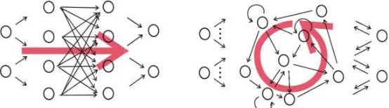
elements information. They perform the same operation for every element in sequence. The neurons are arranged in layers. A system assign weights to connection of neurons and calculates the flow of through the network. According to [5], recurrent networks can be very sensitive, and can adept to past inputs. This makes RNN a robust learning algorithm. One of RNN advantage as machine learning is that their potential for dealing with two sorts of temporal behaviors. RNN is capable of solving complex set of problems and used extensively in many domains to solve compound real-world problems.
Fig 1: Structure of a feed forward network (left) and a recurrent network (right)
C. Attributes of Brokerage Data:
The data set is provided by AlgoAnalytics Financial Consultancy Pvt. Ltd. The indices of brokerage data included total 34 features i.e. input variables and target variables. Target is categorical variable. It gives the state of customers either active or dormant. State of customers is derived from trades done by customer in last three months.
III.PROPOSEDALGORITHM
A. RNN, RFC Ensemble Model based on PAA:
B. Data pre-processing
Step 1: Unreal values are eliminated. Lack of values are compensated firstly in order to clean the data. Then, some unimportant attribute such as city is removed.
Step 2: The time window for train data begins from November 2014 to October 2015. The targeted variables are from November 2015 to January 2016. Time window of test data begins from February 2015 to January 2016. The targeted variables of test data are from February 2016 to April 2016.
Step 3: training data set has 151829 samples and testing data set has 150304 samples.After analyzing training data set, it is observed that 64832 customers are active and others are active within three months. Train and test data set has large number of samples satisfying the conditions of RNN learning. The RNN model is build and trained on training data set and accuracy is predicted using test data.
Step 4: Train data samples values are normalized by:
=
−
−
The values x_new Є [0,1] after normalization. Target = 0 are called as dormant customers and target = 1 are called as active customers.
C. Selection of Principal Attribute:
Principal attributes are selected by calculating the kappa value for each attribute using RNN model. Some attributes kappa value is shown in Table1
TABLE 1.THE KAPPA VALUE AND ATTRIBUTES
Attribute Kappa Value
x1 0.5662
x2 0.5301
x3 x10.5262
x4 0.51
x5 0.4637
x6 0.4312
TABLE 2.BROKERAGE DATA SAMPLES FOR CUSTOMER CHURN ANALYSIS
ID Attributes Active/ Dormant
X1 X2 X3 X4 x5 Target
2 0.6284 664.375 960.295 72.421 35 1
13 1.823 911.853 11.233 1.994 4 1
17 0.556 0 381.703 0 0 1
32 0 126.111 0 0.556 1 0
38 2.567 791.285 0 69.901 19 1
56 1.259 0 66.826 2.238 7 1
83 0 954.905 0 5.910 0 0
181 0 891.148 56.004 0 14 0
224 5.692 0 721.47 52.280 17 1
IV.ENSEMBLE RESULTS
The whole experimental analysis in performed in python programming language using TensorFlow library. The training data set is normalized and RNN, RFC models are trained using training data. The test samples active or dormant are predicted using these models. Other classification algorithms such as SVM are used to predict test data labels in order to compare to the RNN, RFC (with PAA). The result is shown in Table3.
TABLE 3.PREDICATION MODELS AND RESULTS
Prediction model
SVM RFC RNN RNN,RFC
Ensemble
Accuracy(%) 67.94 79.88 81.06 85.65
Kappa value 0.3938 0.5807 0.6028 0.6938
TP 53555 44956 44704 45252
TN 48573 75107 77145 83489
FP 42293 15759 13721 7377
FN 5883 14482 14734 14186
True positive rate(%)
90.10 75.63 75.21 76.13
False positive
rate(%) 46.54 17.34 15.10 8.11
Since there are two categories namely active and dormant customers, four possibilities can be defined to measure the effectiveness of the models.
dormant and consequently lead to a higher churn rate. In the same token, it is important to maximize the TP and TN. Maximizing TP and TN will automatically minimize FP and FN.
Accuracy: (TN+TP)/ (TN+FP+ FN+ TP) True positive rate: TP/ (FN+TP) False positive rate : FP/ (TN+ FP)
It is tested and proved that RNN, RFC ensemble model outperforms SVM, decision tree and RNN. Although difference in performance metrics values may be relatively low, note that even a small gain in prediction performance can yield considerable cost savings for financial firms.
V. CONCLUSION AND FUTURE WORK
In this work, we have surveyed different classification models for churn analysis. RNN, RFC ensemble model of customer churn for brokerage data is suggested because both models runs efficiently on large data sets. In general, ensemble has produced the better results using PAA, which leads to better cost savings in churn applications.On the other hand, comparing to SVM, higher dimension of data samples has lower accuracy and requires more computing time than RNN, RFC.
REFERENCES
1. John Hadden, Ashutosh Tiwari, Rajkumar Roy and Dymitr Ruta (2007), Computer Assisted Customer Churn Management: State-Of-The-Art and Future Trends, Computers & Operations Research v34(10) October 2007, pp2902-2917
2. Zhao Yu, Li Bing, Li Xiu, “Customer churn analysis based on improved support vector machine”, Computer Integrated Manufacturing Systems, 2007, Vol. 13, No. 1, pp. 202-207.
3. MOZER M C, WOLNIEWICZ R, GRIMES D B, et al, “Churn reduction in the wireless industry”, Advances in Neural Information Processing Systems, 2000, pp. 935-941.
4. Department of Computer Science , Carnegie Mellon University Pittsburgh (2009), Dynamic Recurrent Neural Network, 2009
5. Mikael Bod ́en (2001), A guide to recurrent neural networks and back propagation, School of Information Science, Computer and Electrical Engineering Halmstad University, November 13, 2001
6. M. C. Mozer, R. Wolniewicz, D. B. Grimes, E. Johnson, and H. Kaushansky, Predicting sub-scriber dissatisfaction and improving retention in the wireless telecommunications industry,
7. Neural Networks, IEEE Trans., vol. 11, no. 3, pp. 690696, 2000. ”A Survey On Data Mining Techniques In Customer Churn Analysis For Telecom Industry” by Amal M. Almana, Mehmet Sabih Aksoy, Rasheed Alzahrani Lazarov and M. Capota, Churn Prediction, TUM Comput. Sci., 2007.
8. W. H. Au, K. C. C. Chan, and Y. Xin, A novel evolutionary data mining algorithm with applications to churn prediction, Evol. Comput. IEEE Trans., vol. 7, no. 6, pp. 532545, 2003.
9. Sheng Zhao-han, Liu Bing-xiang, “Research method of customer churn crisis based on decision tree”, Journal of Management Sciences in China, Vol. 8, No.2, pp. 20-25,Apr. 2005.
10. Sivasree M S, Rekha Sunny T, Loan Credibility Prediction System Based on Decision Tree Algorithm, International Journal of Engineering Research & Technology (IJERT), September 2015.
BIOGRAPHY