THE NUMERICAL SOLUTION OF THE BAGLEY-TORVIK EQUATION BY EXPONENTIAL INTEGRATORS

Sharif University of Technology

Transactions B: Mechanical Engineering www.scientiairanica.com

The numerical solution to the Bagley-Torvik equation

by exponential integrators

S. Esmaeili

Department of Applied Mathematics, University of Kurdistan, P.O. Box 416, Sanandaj, Iran. Received 30 May 2016; received in revised form 9 July 2016; accepted 29 October 2016

KEYWORDS Fractional derivatives; Fractional dierential equations;

Bagley-Torvik equation; Mittag-Leer function; Exponential integrators.

Abstract. This paper presents a family of computational schemes for the solution to the Bagley-Torvik equation. The schemes are based on the reformulation of the original problem into a system of fractional dierential equations of order 1/2. Then, suitable exponential integrators are devised to solve the resulting system accurately. The attainable order of convergence of exponential integrators for solving the fractional problem is studied. Theoretical ndings are validated by means of some numerical examples. The advantages of the proposed method are illustrated by comparing several existing methods.

© 2017 Sharif University of Technology. All rights reserved.

1. Introduction

Studying fractional calculus is an old topic in math-ematical analysis, which goes back to Leibniz (1695) and Euler (1730) (cf. [1, Section 1.1]). Even though the topic of fractional calculus has a long history, it, however, has drawn the attention of mathematical communities and of specialized conferences only in the last 40 years. Due to new developments in the analysis and understanding of many complex systems in engineering and science elds, it has been observed that several phenomena are more realistically and accu-rately described by dierential equations of fractional order. The well-known anomalous diusion process is one of the most typical examples. Other applications of fractional calculus are linear viscoelasticity, electrical circuits, nuclear reactor dynamic, electrochemistry or image processing (cf. [2-8]).

The operator of fractional derivative is more

*. Tel./Fax: +98 87 33624133

E-mail address: [email protected] doi: 10.24200/sci.2017.4503

complicated than the classical one. As a result, its calculation is also more dicult than the integer order case. Unlike integer order derivatives, which are local operators, the presence of integral in non-integer order derivatives makes the problem global. For this reason, fractional derivatives are powerful tools to describe processes with memory eects and long-range disper-sions. On the other hand, the presence of a signicantly persistent memory, with respect to the integer order case, adds more complexity to the numerical treatment of the related dierential problems, especially for long-time integration.

Since few of the Fractional Dierential Equations (FDEs) encountered in practice can be solved explicitly, it is necessary to employ numerical techniques to nd the approximate solution (cf. [2,6,9]).

One of the numerical methods that has become increasingly applicable in recent years is exponential integrators (cf. [10-12]). Exponential Integrators (EIs) are a class of powerful methods specically designed for solving semi-linear ordinary dierential equations. Basically, the linear term is separated and solved by a matrix exponential and a time-stepping technique is applied to the nonlinear term (cf. [13]). Even though

EIs were introduced in the early 1960s, they have re-ceived little attention in the past due to the diculty in evaluating functions with matrix arguments. In recent years, the spread of ecient methods for performing this task has renewed interests in EIs (cf. [14]).

The seminal paper of Torvik and Bagley (cf. [15]) rst proposed the Bagley-Torvik equation. It has an outstanding role of being a model of motion of a rigid plate immersed in a Newtonian uid. The stability and asymptotic properties of the homogeneous Bagley-Torvik equation are discussed in [16]. Numerical schemes for the Bagley-Torvik equation have been developed in the past ten to fteen years and it has been studied in numerous papers. In [17], the Bagley-Torvik equation is solved by rst reducing this equation to a system of FDEs of order 1/2, and then fractional linear multistep methods and a predictor-corrector method of Adams type are used. Lately, the Bagley-Torvik equation has been numerically solved by hybrid functions approximations [18], a well-posed Chebyshev Tau method [19], the Haar wavelet operational ma-trix [20], and the Bessel collocation method [21]. For further analytical and numerical methods, readers are referred to [22-28].

The main goal of this paper is to design ef-cient numerical schemes for numerical solution to the Torvik equation. To do this, the Bagley-Torvik equation is rst transformed into a system of linear FDEs of commensurate order 1/2, and then by means of the variation-of-constants formula, the exact solution to this problem is obtained. This exact solution does not necessarily provide the best way to compute the solution numerically. Indeed, it typically contains two diculties: evaluating the Mittag-Leer functions with matrix argument and performing the integration analytically. Under certain circumstances, the matrix coecient has eigenvalue de-composition and the rst diculty can be removed. Since most of such integrals cannot be evaluated explicitly, EIs can be used to overcome the second diculty. The resulting method provides promising results. Compared to classical approaches, the polynomial approximation is not applied to the whole vector eld or to the solution of the FDEs, which is a source of inaccuracy in fractional order problems, but just to the external source term that is usually suciently smooth, and hence can be approximated in a satisfactory way by means of polynomials.

The structure of the paper is as follows. In the next section, a brief summary of fractional operators and related special functions is given. In Section 3, the derivation of the Bagley-Torvik equation is rst briey recalled, and then this equation as a system of FDEs of order 1/2 is reformulated. In Section 4, EIs for fractional problem are devised and a description of the proposed numerical scheme is provided. In Section 5,

the convergence properties are studied. Finally, the numerical results demonstrating the eciency of the proposed method are presented in Section 6.

2. Mathematical preliminaries

In this section, some of the main ideas about basic concepts, which will be used later in this paper, are sketched.

2.1. Fractional derivatives

There are many denitions of fractional derivatives (cf. [2,6]); the two most commonly used denitions are those referred to as Riemann-Liouville and Caputo. Their denitions are presented here.

Let 0 and m = de be the smallest integer, such that m > . In mathematical treatises on FDEs, the Riemann-Liouville approach to the notion of the fractional derivative of order and with the starting point at t = 0 is normally used:

0Dty(t) := DmJ0m y(t); t > 0; (1)

where Dm_{denotes the classical dierential operator of}

integer order m and for locally integrable function y: J

0y(t) := ₍₎1

Z _t

0(t s)

1_y(s)ds;

is the Riemann-Liouville fractional integral of order ( > 0).

It is well known that dierential operator D_has

an m-dimensional kernel; therefore, there is certainly a need to specify m initial conditions in order to obtain a unique solution to the straightforward form of a FDE:

D_{y(t) = f(t; y(t));}

with some given function f (cf. [29]). As to the initial value problem for FDEs with the fractional derivatives in the Riemann-Liouville sense, there are some troubles with the initial conditions (cf. [2,30]). Namely, these initial conditions are in the form of:

0D kt y(0) = bk; k = 1; ; m 1;

lim

t!0+J m

0 y(t) = bm;

with given values, bk. However, it is not clear what the

physical meaning of a fractional derivative of y is, and hence it is also not clear how such a quantity can be measured.

A certain solution to this conict was introduced by Caputo and later adopted by Caputo and Mainardi in the framework of the theory of linear viscoelastic-ity (cf. [2,5,9]). Caputo's denition can be written as follows:

D

However, the situation is dierent when dealing with Caputo derivatives. These conditions have the form of:

Dk_{y(0) = c}

k; k = 0; 1; ; m 1;

where real numbers ck are assumed to be given.

As a consequence of denitions (1) and (2) at case 2 N, these fractional derivatives coincide with the classical integer order derivatives (cf. [2,9]). It is well known that the fractional derivatives of Riemann-Liouville and Caputo type are closely linked by the following relationship:

D

y(t) =0Dt[y(t) Tm 1(t)]; (3)

where Tm 1 denotes the Taylor polynomial of degree

m 1 for function y, centered at t = 0.

In order to approximate fractional derivatives, a number of methods have been proposed (cf., e.g., [6,31]).

2.2. Generalized Mittag-Leer functions The Mittag-Leer (ML) function plays a fundamental role in fractional calculus. The ML function with two parameters , 2 C is dened by means of the series expansion:

E;(z) = 1

X

k=0

zk

(k + ); <() > 0:

The relevance of this function appears nowadays in cer-tain fractional relaxation and diusion phenomena [32]. Indeed, the eigenfunction of a FDE, i.e. the solution to the linear test equation D

y(t) = y(t), can be

expressed in terms of the ML function as y(t) = E;1(t)y0, where y(0) = y0 is the initial value.

Recent developments in the solution of FDEs involve a generalization of ML functions, namely:

e;(t; ) = t 1E;(t); t > 0; 2 C;

which plays an important role in the analytical solution of FDEs. In some situations, it is of practical value to scale time variable, t, according to the equivalence:

e;(t; ) = h 1e;(t=h; h); h > 0; (4)

whose proof can be easily derived by using the series representation of ML function, E;. The Laplace

transform of e;(t; ) is (cf. [2,(1.80) for k = 0]):

E;(s; ) = _ss ; <(s) > 0; js j < 1:

An eective way to compute e;(t; ) is by

approx-imating the inversion Laplace transform formula as follows:

e;(t; ) = _2i1

Z

Ce st_E

;(s; )ds;

where contour C is a suitable deformation of the Bromwich line. Based on this approach, the corre-sponding MATLAB code is made freely available (cf. [33]).

The following results on the integration of e;

function will be used later (cf. [2]).

Lemma 2.1. Suppose that t 0, <() > 0, and > 0, and let r 2 R be such that r > 1. Then:

Z _t

0 e;(t s; )s

r_{ds = (r + 1)e}

;+r+1(t; ):

Lemma 2.2. Suppose that a < b t, <() > 0, and > 0. Then:

Z _b

ae;(t s; )ds=e;+1(t a; ) e;+1(t b; );

and: Z _b

a e;(t s; )(s a)ds = e;+2(t a; )

(b a)e;+1(t b; ) e;+2(t b; ):

This section ends with a brief discussion of linear FDEs. Let us consider the following initial value problem, on 0 < < 1, containing a linear FDEs with constant coecients:

D

u(t) = u(t) + g(t); u(0) = u0; (5)

where u(t) : [0; T ] ! R and source term g(t) is assumed to be suciently smooth. Using the Laplace transform (cf. [2, (2.253)]), the desired solution to Problem (5) can be expressed as follows:

u(t) = e;1(t; )u0+

Z _t

0 e;(t s; )g(s)ds:

2.3. Use of matrix functions

Let A be a real or complex square matrix of order m. From elementary linear algebra, there exists non-singular matrix Z, such that:

Z 1_{AZ = diag (J}

1; J2; ; Jp); (6)

where Jk is called a Jordan block of size mk with

eigenvalue k of algebraic multiplicity mk and m1 +

m2+ + mp = m. Suppose that function f is dened

on the spectrum of A, then:

f(A) = Zdiag (f(J1); f(J2); ; f(Jp))Z 1;

where f(Jk) is the upper triangular Toeplitz matrix

is its strictly upper bi-diagonal part by the obtained Taylor series expansion:

f(Jk)=f(k)I +f0(k)Nk+ +f

(mk 1)(

k)

(mk 1)! N mk 1

k ;

since all powers of nilpotent matrix Nk from the mkth

onwards are zero (cf. [14]).

In the case of diagonalizable matrices, the prob-lem becomes very simple and Jordan form (6) reduces to an eigenvalue decomposition:

A = XX 1_{; (7)}

where = diag (1; 2; ; m) and the columns

of matrix X 2 Cmm _{contain linearly independent}

eigenvectors of A. Then:

f(A) = Xdiag (f(1); f(2); ; f(m))X 1;

and hence, just the values of function f on scalar arguments have to be computed.

3. Problem statement

The structural equations of motion dier from the classical formulations as fractional order derivatives are used to model the viscoelastic-damping phe-nomenon (cf. [34]). Bagley commonly attributes the beginning of the modern uses of fractional calculus in linear viscoelasticity to the 1979 PhD thesis under su-pervision of Professor Torvik (cf. [5,35]). To construct the desired model, the main ideas developed in [2,15] will be followed.

A Newtonian uid with density and viscosity , initially at rest, is considered, and it permits the plate at the boundary to commence a general transverse motion. Let (t; z) and v(t; z) be the stress and transverse uid velocity elds, respectively, which are functions of time t and distance z from the uid-plate contact boundary. It is known that (cf. [15, (13)]) the unusual relationship between (t; z) and v(t; z) is as follows:

(t; z) =pD1=2v(t; z): (8)

The physical interpretation of Relationship (8) is that stress at a given point at any time is dependent on the time history of velocity prole at that point.

Let us now consider a rigid plate of mass M and area S immersed in a Newtonian uid of innite extent and connected by a massless spring of stiness K to a xed point. The system is depicted in Figure 1. Force f(t) is applied to the plate, and we nd the dierential equation describing displacement y(t) of the plate to be:

My00_{(t) = f(t) Ky(t) 2S(t; 0):}

Substituting the stress from Eq. (8) and using v(t; 0) =

Figure 1. An immersed plate in a Newtonian uid [2].

y0_{(t), the following FDE is obtained:}

My00_(t)+2Sp_D3=2

y(t)+Ky(t)=f(t); t>0:

A similar equation according to the Riemann-Liouville approach can be obtained. In this case, displacements y(t) and velocities v(t; 0) of the plate uid system must be initially zero (cf. [2, (8.19)]).

As usual, equations of this type are called Bagley-Torvik equation [2,17]. This paper deals with the numerical solution to the following Bagley-Torvik equa-tion:

y00_{(t) + bD}3=2

y(t) + cy(t) = f(t); 0 t T; (9)

with the initial conditions:

y(0) = Y0; y0(0) = Y00; (10)

where Y0 and Y00 are arbitrary real numbers. An

analytical solution for homogeneous initial conditions (Y0= Y00= 0) can be given in the form of:

y(t) = Z _t

0 G(t s)f(s)ds; (11)

with Green function: G(t) =

1

X

k=0

( 1)k

k! ckt2k+1E1=2;2+3k=2(k) ( b

p t);

where E_;(k) is the kth derivative of the ML function (cf. [2, (8.26)]) given by:

E_;(k)(z) =X1

j=0

(j + k)!zj

j! (j + k + ):

This analytical solution includes the evaluation of a convolution integral, which is comprised of a Green's

function stated as an innite sum of derivatives of ML functions, and this cannot be evaluated easily for general functions f. For inhomogeneous initial conditions, expressions that are even more sophisti-cated arise (cf. [17]). The diculty of obtaining an analytical solution was a motivation to investigate numerical schemes for the solution of Eq. (9) with initial conditions Eqs. (10) under which it can be performed more eciently.

Before coming to the description of our numerical scheme, it would be convenient to rewrite the original Bagley-Torvik equation (Eq. (9)) in the form of a system of FDEs of order 1/2 that will later be solved numerically. In particular, the system to be considered is of the following form:

D1=2y0(t) = y1(t);

D1=2y1(t) = y2(t);

D1=2y2(t) = y3(t);

D1=2y3(t) = cy0(t) by3(t) + f(t); (12)

with the initial conditions: y0(0) = Y0; y1(0) = 0;

y2(0) = Y00; y3(0) = 0: (13)

In this context, a useful result, which can nally help us implement EIs, is presented in the following Theorem (cf. [17]).

Theorem 3.1. The Bagley-Torvik (Eq. (9)) with initial conditions (Eqs. (10)) is equivalent to the sys-tem of Eqs. (12) together with the initial conditions (Eqs. (13)) in the following sense:

1. Whenever [y0; y1; y2; y3]T with y0 2 C2[0; T ] for

some T > 0 is the solution to the initial value problems (Eqs. (12) and (13)), function y := y0

solves the initial value problem (9)-(10);

2. Whenever y 2 C2_{[0; T ] is a solution to the initial}

value problem (9)-(10), vector-valued function Y := [y0; y1; y2; y3]T := [y; D1=2 y; y0; D3=2y]T satises the

initial value problem (12)-(13).

Thus, an equation of the following type can be obtained:

D1=2Y(t) = AY(t) + F(t); Y(0) = Y0; (14)

with a given vector-valued function F(t) = [0; 0; 0; f(t)]T_{, unknown solution Y, initial condition vector}

Y0 = [Y0; 0; Y00; 0]T, and 4 4 matrix A of constants

are as follows: A =

2 6 6 4

0 1 0 0 0 0 1 0 0 0 0 1 c 0 0 b

3 7 7 5 :

It would be interesting to justify the reason why y1(0)

and y3(0) can be assumed equal to 0. Indeed, by

means of Eqs. (2) and (12), the following results will be obtained:

y1(t) = D1=2y0(t) = J01=2y0(t);

y3(t) = D3=2y0(t) = J01=2y00(t):

Since y0 _{and y}00 _{are continuous functions, integrals}

J₀1=2y0_{(t) and J}1=2

0 y00(t) vanish for t ! 0 (cf. [17,

Lemma 2.2]).

Hence, by an argument similar to that used for scalar case (Eq. (5)), the exact solution of Eq. (14) at time t is provided by the familiar variation-of-constant formula:

Y(t) = e1=2;1(t; A)Y0+ t

Z

0

e1=2;1=2(t s; A)F(s)ds:

(15) Formula (15) of the exact solution of Eq. (14) is usually considered just as a theoretical tool and is disregarded for practical computation due to the diculty of integration and of evaluating the ML function with matrix arguments. Therefore, numerical solution is the best approach to overcoming these diculties.

4. Exponential integrators for fractional problem

Constructing a class of fractional EIs for Eq. (14) in the spirit of [10,11,12] can be the starting point. The general idea can be as follows. For simplicity, uniform grid points tn = nh, n = 0; 1; , where h > 0 is the

step size is assumed. Eq. (15) is written in the piecewise manner as follows:

Y(tn) =e1=2;1(tn; A)Y0

+n 1X

j=0

Z _tj+1

tj

e1=2;1=2(tn s; A)F(s)ds: (16)

An EI results from Eq. (16) if F(s) is expressed approximately by a linear combination of values at some grid points selected from interval [t0; tj+1]. A

simple way to do this is to approximate F(s) by the unique polynomial interpolating F(s) at such points. This will be implemented in two dierent ways, which

do not suer from restrictions on the step-size due to stability requirements. It has been proved that the stability of this approach is unconditionally guaranteed for methods based on polynomials of degree not greater than 2 (cf. [36]). The resulting discretization scheme involves the evaluation of ML functions on matrix arguments and is performed after diagonalizing the matrix of the system. Due to the small dimension of the systems, the latter task does not appear to be ill-conditioned.

4.1. Fractional exponential Euler scheme In this section, a fairly simple algorithm for numer-ical computation of Eq. (16) is described. In each subinterval [tj; tj+1], vector eld F(s) is approximated

by constant value Fj := F(tj). The application of

Lemma 2.2 into Eq. (16) leads to: Yn= e1=2;1(tn; A)Y0+

n 1

X

j=0

Wn;jFj; (17)

where Yn stands for the approximation of Y(tn) and

weights Wn;j are matrix functions dened as follows:

Wn;j= e1=2;3=2(tn tj; A) e1=2;3=2(tn tj+1; A):

The evaluation of weights Wn;j in EI (Eq. (17))

involves the computation of ML functions with matrix arguments. It is well known that this is not a trivial task.

A simple implementation of Eq. (17) is proposed. Given A in its eigenvalue decomposition (7), after putting Zj = X 1Yj and Gj = X 1Fj, Eq. (17) can

be equivalently written as Yn= XZn with:

Zn= e1=2;1(tn; )Z0+ Wn;0G0+ n 1_X j=1

Wn;jGj

= e1=2;1(nh; )Z0+ e1=2;3=2(nh; )G0

+n 1X

j=1

e1=2;3=2((n j)h; )rGj;

where rGj = Gj Gj 1 are the classical backward

dierences. Then, Eq. (4) yields: Zn= e1=2;1(n; D)Z0+ h1=2

n 1_X j=0

W_{n j}(1) rGj; (18)

with rG0= G0, D = h1=2, and:

W(1)

n = e1=2;3=2(n; D):

4.2. Fractional exponential trapezoidal scheme Given Eq. (16), the scheme can be obtained by employ-ing the piecewise rst-order interpolatemploy-ing polynomials:

P1(s) := Fj+_h1(s tj)rFj+1;

and replacing F(s) by P1(s) when s 2 [tj; tj+1]. Then:

Yn=e1=2;1(tn; A)Y0

+

n 1

X

j=0 tZj+1

tj

e1=2;1=2(tn s; A)Fjds

+_h1n 1X

j=0 tj+1

Z

tj

e1=2;1=2(tn s; A)(s tj)rFj+1ds:

As before, by using Lemma 2.2, the exponential trape-zoidal scheme can be obtained as follows:

Yn=e1=2;1(tn; )Y0

+1_h 0

@f_W0F0+n 1X

j=1

f

Wn;jFj+ fWnFn

1

A ; (19) with weights:

f

W0=e1=2;5=2(tn 1; A) + he1=2;3=2(tn; A)

e1=2;5=2(tn; A);

f

Wn;j=e1=2;5=2(tn tj+1; A) 2e1=2;5=2(tn tj; A)

+ e1=2;5=2(tn tj 1; A);

f

Wn= e1=2;5=2(t1; A):

The resulting explicit scheme is given for n 2 by: Zn=e1=2;1(n; D)Z0

+ h1=2

0 @W(2)_G

0+ n 1

X

j=1

W_{n j}(2) Gj+W0(2)Gn

1 A ;

(20) where, as before, D = h1=2 _and:

W(2) n =

8 > > > > < > > > > :

e1=2;5=2(1; D) n = 0;

e1=2;5=2(n 1; D)

2e1=2;5=2(n; D)

+ e1=2;5=2(n + 1; D)

n 1: and:

W(2)_=e

1=2;5=2(n 1; D) + e1=2;3=2(n; D)

4.3. A particular case

Here, a particular case of right-hand side function, f(t), in Eq. (9) can be considered, where f(t) can be expressed in terms of powers of t. Indeed, given that:

f(t) =X

2J

ct;

with J f 2 R; > 1g an index set and c some

real coecients the exact solution of System (14) can be expressed by means of Lemma 2.1 as follows:

Y(t) =e1=2;1(t; A)Y0

+X

2J

c ( + 1)e1=2;3=2+(t; A)e4: (21)

Here, e4 is the fourth vector of the canonical basis of

R4_{. One of the most obvious advantages of exploiting}

Eq. (21) for practical computation is overcoming sta-bility issues, and the problem is indeed solved in an almost exact way with providing satisfactory results in the presence of stiness as well. Another important success related to the proposed approach is that the numerical solution can be directly evaluated at any given time, t, without the need for approximating the corresponding values at previous time points.

5. Error analysis

In this section, the convergence of the fractional Exponential Euler Scheme (EES) with the fractional Exponential Trapezoidal Scheme (ETS) is proved. In addition, the attainable order of convergence is studied. To express this theme, rst, the following auxiliary lemma is presented (cf. [37]).

Lemma 5.1. Let g(x) = (1 x)_{k(x), where > 1}

and k 2 C([0; 1]). The general trapezoidal quadrature rule:

Q n[g] = 1_n

n

X

j=1

g

2j 1 + 2n

; jj < 1; approximates integral I[g] =R₀1g(t)dt with an error:

Q

n[g] I[g] = ₂k(0)n 1+ O(n 1):

The convergence of fractional EES can be proved by the same kind of ideas developed in [10,11].

Theorem 5.2. Let f 2 C1_{([0; T ]). Then, the}

numerical solution provided by the fractional EES converges with order p = 1. More precisely, error

En := Yn Y(tn) of fractional EES (Eq. (17)) is

expressed as:

En =h₂e1=2;3=2(tn; A)F0(tn) + O(h3=2);

2 (0; 1):

Proof. Subtract the true solution in Eq. (16) from Eq. (17), so the error can be written as follows:

En = n 1_X j=0

Z _tj+1

tj

e1=2;1=2(tn s; A)(Fj F(s))ds:

Applying the change of variable s = tj+ h, scaling

Eq. (4) and the Taylor's theorem, the error is obtained as follows:

En =h3=2 n 1_X j=0

Z ₁

0 e1=2;1=2(n j ; A)(1 )

F0_(t

j+ h)d + O(h5=2):

Using the series expansion dening the ML function: En =h3=2

1

X

k=0

hk=2_Ak

( + 1) Z 1

0 (1 ) n 1_X j=0

(n j )

F0_(t

j+ h)d + O(h5=2);

where = (k 1)=2. Using Lemma 5.1 the following result is obtained:

n 1_X j=0

(n j )_F0_(t j+ h)

=nXn j=1

1 j 1 + _n

F0_{((j 1 + )h)}

=n+1Z 1 0 (1 )

_F0_(t n)d

+ n1

2

F0_{(0) + O(1):}

Applying the integral term mean value theorem to the integral term, the following result is obtained:

n 1_X j=0

(n j )_F0_(t

j+ h) = n +1

+ 1F0(tn)

+ n1

2

F0_{(0) + O(1);}

with 2 (0; 1). Thus, the expansion of error En can

En= h₂ 1

X

k=0

t(k+1)=2n Ak

((k + 3)=2)F0(tn)

+h₁₂2

1

X

k=0

t(k 1)=2n Ak

((k + 1)=2)F0(0) + O(h3=2)

=h₂e1=2;3=2(tn; A)F0(tn)

+h₁₂2e1=2;1=2(tn; A)F0(0) + O(h3=2);

and the proof is complete.

Corollary 5.3. Suppose that f 2 C1_{([0; T ]) and y} n,

n = 1; ; N, as the numerical solution provided by fractional EES. Then:

jy(tn) ynj Ch; n = 1; ; N;

with N = bT=hc and C as a suitable constant which does not depend on h and n.

A similar error estimation procedure for the solu-tion of fracsolu-tional ETS can be currently proposed. Theorem 5.4. Let f 2 C2_{([0; T ]). Then, the}

numerical solution provided by the fractional ETS converges with order p = 2. More precisely, error En := Yn Y(tn) of fractional ETS (Eq. (19)) is

expressed as follows: En= h

2

12e1=2;3=2(tn; A)F00(tn) + O(h5=2); 2 (0; 1):

It should be noted that the proof of Theorem 5.2 can be adopted without diculty to deal with Theorem 5.4. Corollary 5.5. Suppose that f 2 C2_{([0; T ]) and y} n,

n = 1; ; N, as the numerical solution provided by fractional ETS. Then:

jy(tn) ynj Ch2; n = 1; ; N;

with N = bT=hc and C as a suitable constant which does not depend on h and n.

This section ends with a brief discussion of the less regular case in which the source term is f f(y(t)). The resulting system is a semi-linear problem as follows:

D

Y(t) = AY(t) + F(Y(t)); Y(0) = Y0:

According to the results in [10], by applying fractional ETS, one should obtain an order of convergence pro-portional to h3=2 _{and not to h}2 _{as stated in the case}

f f(t) in Theorem 5.4. Indeed, a drop in the order of convergence is expected, since y(t) and f(y(t)) are usually singular at the origin. Thus, the main advantage of the use of EIs for FDEs is indeed not just conned to stability, but is also related to the improvement of the order of convergence when linear systems are solved.

6. Results and discussion

In this section, some numerical studies are presented to illustrate and test the behavior of the approach described in Section 4. All the algorithms are imple-mented in Matlab and the evaluation of scalar ML function on the spectrum of coecient matrix A is performed by the Matlab code ml from [33]. Since we were originally interested in the solution of the given scalar the initial value problem (9)-(10), there is a need to look at the rst component of solution vector Y. Example 1. As a rst example, we choose f(t) so that the exact solution to the initial value problems (9)-(10) is y(t) = t_{. It can be checked that the}

corresponding forcing term is as follows: f(t) = ( 1)t 2₊ b ( + 1)

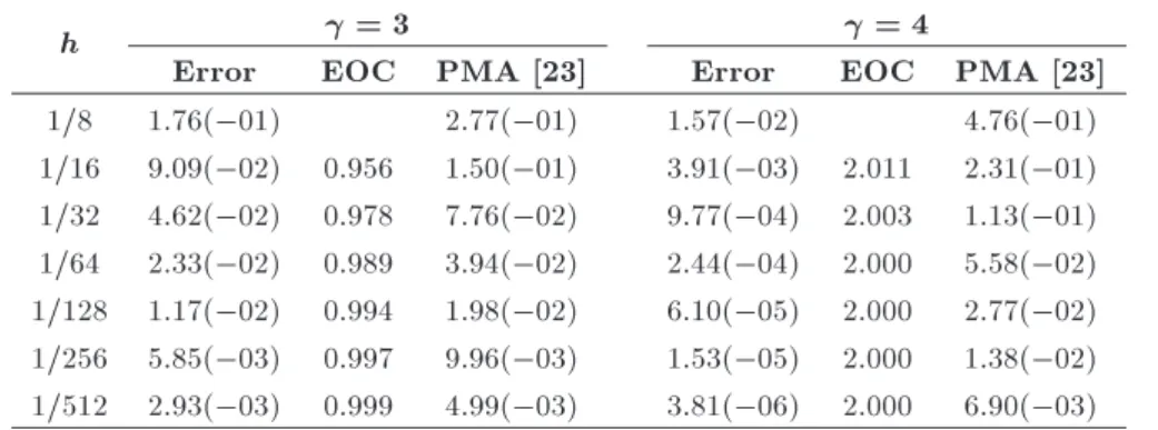
( 1=2)t 3=2+ ct: The numerical solution is evaluated at t = 1 according to the fractional EES and the fractional ETS by a sequence of decreasing step size h. Errors e(h), with respect to the exact solution, together with an exper-imental order of convergence, denoted with EOC and obtained as log₂(e(h)=e(h=2)), are reported in Table 1. The close agreement of the empirical values of EOC with the theoretically predicted values of 1 and 2 can be seen, respectively. In addition, the absolute errors are compared with the Podlubny's Matrix Approach (PMA) in [23].

Example 2. The initial value problem (9)-(10) with b = p are considered, in which is a parameter, c = 1, Y0 = 1, Y00 = 0, and f(t) 0. This

mathematical model is developed for a micro-electro-mechanical system instrument, designed primarily to measure the viscosity of uids encountered during oil well exploration. As mentioned in [38], the solution reduces to cos t, as ! 0, as illustrated. Since F 0, then Y(t) = e1=2;1(t; A)Y0, by means of Eq. (15). The

numerical solutions for various parameter and T = 30 are plotted in Figure 2 and are reported in Table 2. Example 3. The most popular initial value prob-lem (9)-(10) can be assumed with Y0= Y00= 0 and:

f(t) = (

8 0 t 1; 0 t > 1:

Table 1. The resulting values of errors, EOC, and PMA at t = 1 for b = c = 1 (Example 1).

h = 3 = 4

Error EOC PMA [23] Error EOC PMA [23]

1/8 1:76( 01) 2:77( 01) 1:57( 02) 4:76( 01)

1/16 9:09( 02) 0.956 1:50( 01) 3:91( 03) 2.011 2:31( 01) 1/32 4:62( 02) 0.978 7:76( 02) 9:77( 04) 2.003 1:13( 01) 1/64 2:33( 02) 0.989 3:94( 02) 2:44( 04) 2.000 5:58( 02) 1/128 1:17( 02) 0.994 1:98( 02) 6:10( 05) 2.000 2:77( 02) 1/256 5:85( 03) 0.997 9:96( 03) 1:53( 05) 2.000 1:38( 02) 1/512 2:93( 03) 0.999 4:99( 03) 3:81( 06) 2.000 6:90( 03) Table 2. The resulting values of EI with = 0:20 in some values of t (Example 2).

t 1 2 5 10 15 20 25 30

y(t) 0.6188 0:1398 0:2436 0:3114 0.2086 0.0330 0:0936 0.0229

Figure 2. Fractional Bagley-Torvik equation (Example 2).

Since Y0 0 by means of Eq. (15) and Lemma 2.2,

Y(t) = 8B(t)e4, where:

B(t)= 8 > < > :

e1=2;3=2(t; A) 0t1;

e1=2;3=2(t; A) e1=2;3=2(t 1; A) t > 1:

Thanks to the work of Cermak and Kisela in [16], the asymptotic behavior of the exact solution is y(t) = O(t 1=2_{) as t ! 1. In Figure 3, the rst component}

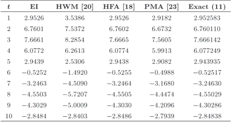
of the solution vector Y(t) for b = c = 0:5, b = c = 1, and T = 30 are illustrated. The resulting values of the present method and some numerical methods for t = 1; 2; ; 10 are also reported in Table 3. It can be seen that the presented method provides closer results to the exact solution than others.

Example 4. The last test is initial value problems (Eqs. (9) and (10)) with b = 2, c = 1, Y0 = 0, Y00 =

1, and f(t) = sin t. Unfortunately, an exact solution to these problems is not available. Thus, a reference solution, the numerical approximation given by PMA in [23] with step sizes h = 0:01, is used. The numerical

Figure 3. Fractional Bagley-Torvik equation: solution by EI (Example 3.)

Figure 4. Numerical solution by EIs and PMA (Example 4).

results of the new method proposed in this paper and PMA with T = 10 are shown in Figure 4 and in Table 4. These results indicate that the approximate solutions of the present method are in agreement with those of the literature reviews.

7. Conclusions

This paper deals with a numerical method to solve the Bagley-Torvik equation using the EIs method. In

Table 3. The resulting values of EI and available methods with b = c = 0:5 (Example 3). t EI HWM [20] HFA [18] PMA [23] Exact (11)

1 2.9526 3.5386 2.9526 2.9182 2.952583

2 6.7601 7.5372 6.7602 6.6732 6.760110

3 7.6661 8.2854 7.6665 7.5605 7.666142

4 6.0772 6.2613 6.0774 5.9913 6.077249

5 2.9439 2.5306 2.9438 2.9082 2.943935

6 0:5252 1:4920 0:5255 0:4988 0:52517

7 3:2463 4:5090 3:2464 3:1680 3:24630

8 4:5503 5:7207 4:5505 4:4474 4:55029

9 4:3029 5:0009 4:3030 4:2096 4:30286

10 2:8484 2:8403 2:8486 2:7939 2:84838

Table 4. The resulting values of EI with h = 0:05 and PMA with h = 0:01 in some values of t (Example 4).

t 1 2 3 4 5 8 9 10

EES 0.9868 1.8907 2.4188 2.2762 1.4744 0:3343 0.0563 0.4257 ETS 0.9877 1.8925 2.4199 2.2750 1.4714 0:3322 0.0589 0.4266 PMA 0.9955 1.8947 2.4145 2.2635 1.4595 0:3207 0.0700 0.4310

particular, the fractional exponential Euler scheme and fractional exponential trapezoidal scheme have been developed to obtain the numerical solution to the Bagley-Torvik equation. The proposed method can be used eectively for the solution of multi-term FDEs so that the Bagley-Torvik equation can serve as one of their prototypes. Implementation issues and error analysis have been treated. The accuracy and validity of the method have been veried by dierent numerical studies.

References

1. Oldham, K.B. and Spanier, J., The Fractional Cal-culus: Theory and Applications of Dierentiation and Integration to Arbitrary Order, Academic Press, New York (1974).

2. Podlubny, I., Fractional Dierential Equations, Aca-demic Press, San Diego, CA (1999).

3. Metzler, R. and Klafter, J. \The random walks guide to anomalous diusion: a fractional dynamics approach", Phys. Rep., 339, pp. 1-77 (2000).

4. Rossikhin, Y.A. and Shitikova, M.V. \Application of fractional calculus for dynamic problems of solid mechanics: Novel trends and recent result", Appl. Mech. Rev., 63(1), pp. 010801-52 (2009).

5. Mainardi, F., Fractional Calculus and Waves in Lin-ear Viscoelasticity: An Introduction to Mathematical Models, Imperial College Press, London (2010).

6. Baleanu, D., Diethelm, K., Scalas, E. and Trujillo, J.J., Fractional Calculus: Models and Numerical Methods, 2nd Ed., World Sci. Publishing, Singapore (2016).

7. Atanackovic, T.M., Pilipovic, S., Stankovic, B. and Zorica, D., Fractional Calculus with Applications in Mechanics: Vibrations and Diusion Processes, Wiley-ISTE, London (2014).

8. Garrappa, R. Mainardi, F. and Maione, G. \Models of dielectric relaxation based on completely monotone functions", Fract. Calc. Appl. Anal., 19(5), pp. 1105-1160 (2016).

9. Diethelm, K., The Analysis of Fractional Dierential Equations, Springer, Berlin (2010).

10. Garrappa, R. and Popolizio, M. \Generalized expo-nential time dierencing methods for fractional order problems", Comput. Math. Appl., 62(3), pp. 876-890 (2011).

11. Garrappa, R. \A family of Adams exponential inte-grators for fractional linear systems", Comput. Math. Appl., 66(5), pp. 717-727 (2013).

12. Garrappa, R. \Exponential integrators for time-fractional partial dierential equations", Eur. Phys. J. Special Topics, 222(8), pp. 1913-1925 (2013).

13. Hochbruck, M. and Ostermann, A. \Exponential inte-grators", Acta Numerica, 19, pp. 209-286 (2010).

14. Higham, N.J., Functions of Matrices: Theory and Computation, SIAM, Philadelphia, PA (2008).

15. Torvik, P.J. and Bagley, R.L. \On the appearance of the fractional derivative in the behavior of real materials", J. Appl. Mech., 51(2), pp. 294-298 (1984).

16. Cermak, J. and Kisela, T. \Exact and discretized

stability of the Bagley-Torvik equation", J. Comput. Appl. Math., 269, pp. 53-67 (2014).

17. Diethelm, K. and Ford, N.J. \Numerical solution of the Bagley-Torvik equation", BIT, 42(3), pp. 490-507 (2002).

18. Mashayekhi, S. and Razzaghi, M. \Numerical solution of the fractional Bagley-Torvik equation by using hybrid functions approximation", Math. Meth. Appl. Sci., 39(3), pp. 353-365 (2016).

19. Mokhtary, P. \Numerical treatment of a well-posed Chebyshev Tau method for Bagley-Torvik equation with high-order of accuracy", Numer. Algorithms, 72(4), pp. 875-891 (2016).

20. Saha Ray, S. \On Haar wavelet operational matrix of general order and its application for the numerical solution of fractional Bagley-Torvik equation", Appl. Math. Comput., 218(9), pp. 5239-5248 (2012).

21. Yuzbas, S. \Numerical solution of the Bagley-Torvik equation by the Bessel collocation method", Math. Meth. Appl. Sci., 36(3), pp. 300-312 (2013).

22. Luchko, Y. and Goreno, R. \An operational method for solving fractional dierential equations with the Caputo derivatives", Acta Math. Vietnamica, 24(2), pp. 207-233 (1999).

23. Podlubny, I. \Matrix approach to discrete fractional calculus", Fract. Calc. Appl. Anal., 3(4), pp. 359-386 (2000).

24. Saadatmandi, A. and Dehghan, M. \A new operational matrix for solving fractional-order dierential equa-tions", Comput. Math. Appl., 59(3), pp. 1326-1336 (2010).

25. Esmaeili, S., Shamsi, M. and Luchko, Y. \Numerical solution of fractional dierential equations with a collo-cation method based on Muntz polynomials", Comput. Math. Appl., 62(3), pp. 918-929 (2011).

26. Jafari, H., Youse, S.A., Firoozjaee, M.A., Momani, S. and Khalique, C.M. \Application of Legendre wavelets for solving fractional dierential equations", Comput. Math. Appl., 62, pp. 1038-1045 (2011).

27. Bhrawy, A.H., Taha M.T. and Machado, J.A.T. \A review of operational matrices and spectral techniques for fractional calculus", Nonlinear Dyn., 81(3), pp. 1023-1052 (2015).

28. Jafari, H., Kdkhoda, N., Azadi, M. and Yaghobi, M. \Group classication of the time-fractional Kaup-Kupershmidt equation", Scientia Iranica, 24(1), pp. 302-307 (2017).

29. Diethelm, K. and Ford, N.J. \Analysis of fractional dierential equations", J. Math. Anal. Appl., 265(2), pp. 229-248 (2002).

30. Podlubny, I. \Geometric and physical interpretation of fractional integration and fractional dierentiation", Fract. Calc. Appl. Anal., 5(4), pp. 367-386 (2002).

31. Esmaeili, S. and Milovanovic, G.V. \Nonstandard Gauss-Lobatto quadrature approximation to fractional derivatives", Fract. Calc. Appl. Anal., 17(4), pp. 1075-1099 (2014).

32. Goreno, R., Kilbas, A.A., Mainardi, F. and Rogosin, S.V., Mittag-Leer Functions, Related Topics and Applications Theory and Applications, Springer, Berlin (2014).

33. Garrappa, R. \Numerical Evaluation of two and three parameter Mittag-Leer functions", SIAM J. Numer. Anal., 53(3), pp. 1350-1369 (2015).

34. Bagley, R.L. and Calico, R.A. \Fractional order state equations for the control of viscoelastically damped structures", J. Guid. Control Dynam., 14(2), pp. 304-311 (1991).

35. Bagley, R.L., Applications of Generalized Derivatives to Viscoelasticity, Air Force Institute of Technology, PhD Dissertation (1979).

36. Lubich, C. \A stability analysis of convolution quadra-tures for Abel-Volterra integral equations", IMA J. Numer. Anal., 6(1), pp. 87-101 (1986).

37. Lyness, J.N. and Ninham, B.W. \Numerical quadra-ture and asymptotic expansions", Math. Comp., 21(98), pp. 162-178 (1967).

38. Fitt, A.D., Goodwin, A.R.H., Ronaldson, K.A. and Wakeham, W.A. \A fractional dierential equation for a MEMS viscometer used in oil industry", J. Comput. Appl. Math., 229(2), pp. 373-381 (2009).

Biography

Shahrokh Esmaeili is an Assistant Professor in the Department of Mathematics at University of Kur-distan. He received his BS degree from Amirkabir University of Technology in 1998 and his MSc degree from Tarbiat Modares University in 2000. He started his doctoral program in 2008 and received his PhD degree from Amirkabir University of Technology in 2011 in Applied Mathematics. His current research interest mainly covers numerical methods for fractional dierential equations.