Neutrality Tests for Sequences with Missing Data

(1)

NOTE

Neutrality Tests for Sequences with Missing Data

Luca Ferretti,*,1,2_{Emanuele Raineri,}†,2_{and Sebastian Ramos-Onsins*}

*Centre for Research in Agricultural Genomics, 08193 Bellaterra, Spain and†_{Centro Nacional de Análisis}

Genómico, 08028 Barcelona, Spain

ABSTRACTMissing data are common in DNA sequences obtained through high-throughput sequencing. Furthermore, samples of low quality or problems in the experimental protocol often cause a loss of data even with traditional sequencing technologies. Here we propose modiﬁed estimators of variability and neutrality tests that can be naturally applied to sequences with missing data, without the need to remove bases or individuals from the analysis. Modiﬁed statistics include the Watterson estimatoruW, Tajima’sD, Fay and Wu’s H, and HKA. We develop a general framework to take missing data into account in frequency spectrum-based neutrality tests and we derive the exact expression for the variance of these statistics under the neutral model. The neutrality tests proposed here can also be used as summary statistics to describe the information contained in other classes of data like DNA microarrays.

N

EUTRALITY tests are among the most widely used tools in population genetics. Many neutrality tests have been developed based on the levels and the patterns extracted from segregating sites, and in particular to be applied to biallelic SNP data. The simplest information that can be extracted from SNP data are the allele frequency spectrum; therefore, many tests focus on the difference between the observed and expected spectrum under the neutral Wright– Fisher model. Widespread tests of this kind include Tajima’s

D(Tajima 1989), Fu and Li’sFandD(Fu and Li 1993), and Fay and Wu’sH(Fay and Wu 2000). However, this class of tests is much larger, as recently shown by Achaz (2009) following an idea of Nawa and Tajima (2008), and includes among the others the tests by Fu (1997), Zenget al.(2006), and Achaz (2009). A subclass of optimal neutrality tests against speciﬁc alternative scenarios was described by Ferretti

et al.(2010). Some general results on the variances of these tests were provided by Fu (1995) and Pluzhnikov and Donnelly (1996).

All these statistics assume a complete knowledge of the alleles present in the n sequenced individuals for all the

Lpositions genotyped. However, this is rarely the case:

ex-perimental problems in sample preparation or genotyping often result in missing data; i.e., some individual alleles at some positions are actually unknown.

At present, most packages for population genetics ana-lyses like DNAsp (Librado and Rozas 2009) deal with missing data simply by removing individuals and/or positions af-fected with incomplete data. This is a good strategy as long as missing data represent a very minor fraction of the alleles, since in this case they do not affect the power of the anal-ysis. However, there could be situations in which a large amount of missing data are unavoidable. For example, in samples taken from natural populations the quality of the samples could be low or the amount of DNA available per individual could be insufﬁcient; therefore, genotyping these samples could miss a signiﬁcant fraction of the alleles.

There is another important reason to consider sequences with missing data. Many of the sequences that are being produced currently are not obtained through Sanger se-quencing, but from next-generation sequencing (NGS) tech-nologies. These technologies sequence a large amount of short reads that are then realigned to reconstruct the original sequence. The coverage of these reads is strongly inhomogeneous along the genome and there is often a large fraction of bases that is not covered by a sufﬁcient number of reads, unless the coverage is very high. Missing data are therefore inherent to these technologies: hence, removing individuals or bases with missing alleles would imply a huge loss of information. Given the growing relevance of NGS technologies for population genetics studies, a different strategy is needed to deal with this circumstance. Several

Manuscript received February 22, 2012; accepted for publication May 24, 2012 Supporting information is available online at http://www.genetics.org/content/ suppl/2012/06/01/genetics.112.139949.DC1.

1_{Corresponding author: Centre de Recerca en Agrigenòmica (CRAG), Campus} Universitat Autònoma de Barcelona, 08193 Bellaterra, Spain.

E-mail: [email protected]

2_{These authors contributed equally to this work.}

(2)

estimators of variability can be applied directly to sequenced reads (Lynch 2008; Hellmannet al.2008; Jianget al.2009; Futschik and Schlötterer 2010; Kang and Marjoram 2011); however, no estimator is available for the sequences ob-tained after genotype call has been completed for each in-dividual in each position. The difference between these two situations is that, once the genotype has been deter-mined, all the information about the single read bases align-ing on a given position and their qualities is (for our purposes) lost.

In this article we present a simple generalization of some estimators and tests that take missing data into account. In particular we consider the Watterson estimator of genetic variability (Watterson 1975), the Tajima estimator of nucle-otide diversity (Tajima 1983), neutrality tests based on the frequency spectrum like Tajima’sDand Fay and Wu’sH, and the HKA test (Hudson et al. 1987) for neutral evolution based on the pattern of polymorphism and divergence. The most important result of this article is the general ex-pression for the covariance between the frequency spectrum at two sites CovðjiðxÞ;jjðyÞÞ, which is the basis for the

com-putation of the variances of the estimators and tests pre-sented here.

Note that in sequence data, missing data (usually rep-resented byN’s located in the same position as the missing alleles) are not equivalent to gaps (represented by white spaces). Gaps correspond to insertions or deletions (indels) in some of the sequences. In this article we do not address indels, even if very short biallelic indels (a few bases long) are similar to SNPs as genetic variants and therefore could be analyzed by similar methods. In practice it is difﬁcult to differentiate indels from missing data if the rate of missing data are high, and this is especially true for sequences obtained from NGS data. Here we consider sequences with-out indels.

Neutrality Tests Including Missing Data

In this article we consider estimators and tests based on the frequency spectrum. The basic population parameter in-volved in these tests is the nucleotide variabilityu= 2Nem,

whereNeis the haploid effective population size andmis the

mutation rate per base per generation. We assume a small variabilityu1 and a large window lengthL1, such that uLOð1Þ.

All the tests and estimators belong to a general class of neutrality tests that can be parametrized in terms of weights vi,Vi(Achaz 2009),

^ u¼1

L X n21

i¼1

iviji; X n21

i¼1

vi¼1 (1)

T¼ ^u2^u9

Varð^u2^u9Þ¼

Pn21

i¼1iViji

VarPn2i¼11iViji

; X

n21

i¼1

Vi¼0; (2)

where jiindicates the number of variants with frequency i

for the derived allele. The weightsvi,Vimultiply the

nor-malized frequency spectrum ui = iji (Nawa and Tajima

2008). The estimators are unbiased estimators of u, while the tests are normalized to have mean 0 and variance 1 under the standard neutral model without recombination.

Our deﬁnition of neutrality tests based on the frequency spectrum is the most general parametrization compatible with Equations 1–2 that takes explicitly into account the coverage for each site. We denote by n the total number of individuals sequenced and bynxthe number of

individu-als for which the allele at positionxis known. The estima-tors and tests are deﬁned as

^ u¼1

L XL

x¼1 X nx21

i¼1

ivi;nxjiðxÞ;

1 L XL x¼1 X nx21 i¼1

vi;nx ¼1 (3)

T¼ ^u2^u9

Varð^u2^u9Þ

¼

PL x¼1

Pnx21

i¼1 iVi;nxjiðxÞ

VarPL_x_¼₁Pnx2_i_¼₁1iVi;nxjiðxÞ

; X

L

x¼1

X nx21

i¼1

Vi;nx ¼0;

(4)

whereji(x) is an index variable that is 1 if there is a

segre-gating site with iderived alleles in positionxand 0 other-wise. The estimators are unbiased, i.e.,Eð^uÞ ¼u, while the tests are normalized toE(T) = 0, Var(T) = 1 as in the usual framework.

The weights vi;nx, Vi;nx deﬁne the speciﬁc estimator

or test (Achaz 2009). The most important estimator of var-iability is the Watterson estimator ^uW¼S=anL; where we

denote by S the total number of segregating sites and

an¼ Pn21

i¼11=i. This estimator can be obtained as a maximum

composite likelihood estimator (MCLE) (Hellmann et al.

2008). Its natural generalization is the MCLE with missing data,

vWi;nx ¼

1

iPL_x_¼1anx=L

⇒ ^uW¼PLS x¼1anx

; (5)

which depends only onS. For most of the other estimators like Tajima’sP, we choose the weightsvi;nxto be simply the

same as the weights vi for the estimators (1), where n is

substituted by nx, that is, vPi;nx ¼2ðnx2iÞ=nxðnx21Þ. This

deﬁnition is equivalent to^uP¼P=L, wherePis the average

pairwise diversity per base, which is naturally deﬁned even with inhomogeneous coverage.

As for neutrality tests, Tajima’sD (Tajima 1989) corre-sponds to ^uP2^uW, that is, to the weights

VD i;nx ¼

2ðnx2iÞ

nxðnx21Þ2

1

iPL_y_¼1any=L

; (6)

and Fay and Wu’sH(Fay and Wu 2000) corresponds to

(3)

VH i;nx ¼

2ðnx2iÞ

nxðnx21Þ2

2i

nxðnx21Þ: (7)

The other tests can be generalized in a similar way. All the tests and estimators reduce to their usual expressions if no data are missing;i.e.,nx=nfor all sites.

In this framework it is also possible to implement error corrections for error-prone data: for example, removing singletons (Achaz 2008) is equivalent to the choice of v1;nx ¼vnx21;nx ¼0 and a rescaling of the other vi;nx to

match the normalization in Equation 3. For NGS data, in-formation on base or SNP qualities is usually available; hence, a more refined error correction strategy consists in weighting each SNP in Equations 3–4 by the probability that it has been correctly identified. A detailed treatment can be found in Supporting Information,File S1. For NGS data it is also useful to filter out the bases with low coverage, i.e., the ones for which information from most individuals is missing. If we assume that the minimum number of individuals covering reliable positions isnmin, thisfilter can be easily implemented

by removing all positions withnx,nminfrom the analysis.

To evaluate the tests (4), we need the variances in the denominators. Our basic result for these variances (leaving out subleading terms inuand 1/L) is

Var X

L

x¼1

X nx21

i¼1 iVi;nxjiðxÞ

! ¼XL

x¼1

X nx21

i¼1 iV2

i;nxuþ

XL

x;y¼1

x6¼y X nx21

i¼1

X ny21

j¼1

ijVi;nxVj;nyCov

jiðxÞ;jjðyÞ

(8)

since ji(x) are index variables with meanE(ji(x)) =u/iand

ji(x),jj(x) are mutually exclusive fori6¼j, soE(ji(x)jj(x)) = 0.

The covariance Cov(ji(x),jj(y)) for the standard neutral model

without recombination is presented in the next section. The HKA (Hudson, Kreitman, Aguadé) test (Hudsonet al.

1987) and the formulae for estimators and tests based on the folded spectrum are treated inFile S1.

Covariance of the Frequency Spectrum at Different Sites

Sinceji(x),jj(y) are index variables, their covariance under

the standard neutral model without recombination is

CovjiðxÞ;jjðyÞ

¼P_ij_ð_nx_;_ny_;_nxy_Þ2u

2

ij; (9)

wherePijðnx;ny;nxyÞis the probability of observing SNPs of

fre-quencyiandj,nxandnyare the numbers of individuals with

known alleles at the two sites, and nxy is the number of

individuals for which both alleles are known. This probabil-ity can be obtained as

P_ij_ð_nx_;_ny_;_nxy_{Þ ¼} X

nxþny2nxy21

k;l¼1

C_ijS_;_kl_ð_nx_;_ny_;_nxy_ÞPS_kl_ð_nx_þ_ny2nxy_Þ

þCE_ij_;_kl_ð_nx_;_ny_;_nxy_ÞPE_kl_ð_nx_þ_ny2_nxy_Þ

; (10)

wherePS

klðnÞ andPEklðnÞare the probabilities of shared (S) or exclusive (E) pairs of mutations of frequency k and l inn

complete sequences. (We deﬁne a pair of mutations as shared if there are individuals with derived alleles in both loci and as exclusive if no individual sequence contains both the derived alleles.) The sumPS

klþPEklgives the probability

for complete sequences Pkl = u2(1/kl + skl), where the

matrixsklis deﬁned in Fu (1995, Equations 2–3).

The coefﬁcients CS_ij;_;E_kl_ð_n

x;ny;nxyÞ represent the probabilities

that, given a pair of shared or exclusive mutations with frequencies k and lin nx +ny 2nxy complete sequences, iandjderived alleles are found among thenx,nyalleles in x and y, respectively, assuming that the nx, ny individuals

(with nxy in common between the two sets) are randomly

extracted from the complete set ofnx+ny2nxyindividuals.

The combinatorial formulae for these probabilities are

CS

ij;klðnx;ny;nxyÞ ¼

_n

x2nxy

l₂j

ny2nxy

k₂i

_n

xþny2nxy

l;k2l;nxþny2nxy2k

X

minði;nx2nxy;k2jÞ

kx¼maxði2nxy;l2jÞ

_n

xy

i₂kx

_n

x2nxyþj2l

kxþj2l

k2kx

j

(11)

ifk$l; otherwise use the identityCS

ij;klðnx;ny;nxyÞ¼C

S

ji;lkðny;nx;nxyÞ,

CE_ij_;_kl_ð_n

x;ny;nxyÞ ¼

_n

x2nxy

l2j

ny2nxy

k2i

_n

xþny2nxy

k;l;nxþny2nxy2k2l

X

minði;nx2nxyþj2lÞ

kx¼maxð0;i2nxy;k2nyþjÞ

_n

xy

i2kx

_n

x2nxyþj2l

kx

ny2kþkx

j ;

(12)

where ð a

b;c;a2b2cÞ is the multinomial coefﬁcient a!=b!c!

ða2b2cÞ!. We deﬁneCS

ij;klðnx;ny;nxyÞorC

E

ij;klðnx;ny;nxyÞ to be zero

if there are negative arguments in the binomial or multino-mial coefﬁcients in the above Equations 11 or 12.

The formulae for the probabilitiesPS_kl;E_ð_n_Þ can be obtained by breaking the derivation ofE(jkjl) by Fu (1995) into the

contributions from shared mutations (Fu 1995, Equations 24 and 28) and exclusive mutations (Equations 25, 29, and 30):

PSklðnÞ¼u2dklbnðkÞ þu2ð12dklÞ

bnðminðk;lÞÞ2bnðminðk;lÞ þ1Þ

2

(13)

PE_kl_ð_n_Þ_¼

8 > > > > > > < > > > > > > : u2 ₁ kl2

bnðkÞ2bnðkþ1Þ þbnðlÞ2bnðlþ1Þ

2

fork_þl_,n

u2

_a n2ak

n2k þ an2al

n2l þ

bnðkÞ þbnðlÞ

2

fork_þl_¼n

0 fork_þl_.n

(14)

(4)

with

an¼ X n21

i¼1

1

i; bnðiÞ ¼

2n

ðn2iþ1Þðn2iÞðanþ12aiÞ2

2

n2i:

(15)

Some special cases of these formulae are treated inFile S1, Figure S1, andFigure S2.

Finally, note that the computation of the variances re-quires an estimate of ^uand^u2. These estimates are usually obtained by the method of moments (MM). In our approach, ^

u is given by the Watterson estimator (5), while the MM estimate of ^u2is given by

^

u2¼ S

2₂_S PL

x¼1anx 2

þPL x;y¼1

Pnx21

i¼1 Pnj¼1y21Cov

jiðxÞ;jjðyÞ

u2

:

(16)

Discussion

In this article we presented a general framework for esti-mators of variability and neutrality tests based on the frequency spectrum that take into account missing data in a natural way. This is particularly interesting in the light of sequences obtained from NGS data, since for these technol-ogies a relevant fraction of bases is often not sequenced or sequenced at very low read depth.

The approach discussed here is based on results that are conditional on the distribution of the missing data, as summarized by the distribution of all the triples (nx, ny, nxy). An effective way of implementing numerically the

above variances is to sample Ns random values of (nx, ny, nxy) from the empirical distribution and compute the

cova-riances using only these values and then rescale the second term in Equation 8 by a factorL2_/_N

s.

The modiﬁcations presented in this article can be applied to all estimators and tests included in the framework of Achaz (2009) and represent, therefore, a complete tool with which to deal with missing data. However, it would be in-teresting to know the impact of the missing data on the performance of the estimators and tests. If weﬁx the sample size, an increase in the amount of missing data leads to an increase in the variance of the estimators (Figure 1), as is to be expected given that this is equivalent to loss of informa-tion. On the other hand, if the loss of information associated with missing data is compensated by sequencing more indi-viduals, the performances of the estimators actuallyincrease

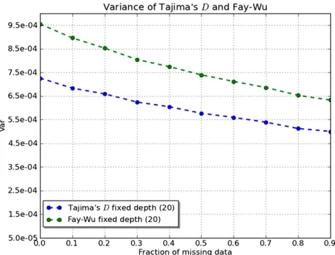
(i.e., their variances decrease) with respect to complete sequences with the same coverage (Figure 1). A similar ef-fect can be observed for neutrality tests (Figure 2). The explanation for this counterintuitive behavior lies in the fact that in the case of complete sequences, all individuals share the same genealogical tree at all positions,i.e., the same evo-lutionary history, while in this case different positions are cov-ered by different sets of individuals with partly independent histories in the same population; therefore, the number of available histories is actually larger and the variance is re-duced similarly to what happens with recombination. Our results imply that with the same amount of information per base, missing data could improve the power of neutrality tests.

Figure 1 Variance of the Watterson estimatoruWon a window ofL=

100 bases foru= 0.1. Computed by drawing out randomlyNs= 100

triples (nx,ny,nxy) in two different ways. First, weﬁx the sample sizen=

20 and remove alleles randomly according to the probabilitypmof

miss-ing an allele (solid blue line). In this case the number of individuals isﬁxed but the actual depth may vary along the sequence. Second, the number of individuals sequenced in each position is adjusted to keep the average depth constant at n(1 2pm) ’ 20 (dashed green line) and then we

remove alleles with probabilitypm. In this case the sample size isn’

20/(12pm).

Figure 2 Variance of Tajima’s D (bottom line) and Fay and Wu’s H

(top line) on a window ofL= 100 bases foru= 0.1. Computed as in Figure 1 for ﬁxed average depth n(1 2 pm) ’ 20. (Note that Fay

and Wu’sHvariance is divided by 4 to appear in scale with Tajima’s

Dvariance.)

(5)

Acknowledgments

Work funded by grant CGL2009-09346 to S.R.O., grant AG2010-14822 to Miguel Pérez-Enciso, and Consolider grant CSD2007-00036 “Centre for Research in Agrigeno-mics” (Ministerio de Ciencia e Innovación, Spain). S.R.O. is recipient of a Ramón y Cajal position (Ministerio de Cien-cia e Innovación, Spain). L.F. acknowledges support from Consejo Superior de Investigaciones Cientíﬁcas (Spain) under the JAE-doc program.

Literature Cited

Achaz, G., 2008 Testing for neutrality in samples with sequencing

errors. Genetics 179: 1409.

Achaz, G., 2009 Frequency spectrum neutrality tests: one for all

and all for one. Genetics 183: 249.

Fay, J., and C.-I. Wu, 2000 Hitchhiking under positive Darwinian

selection. Genetics 155: 1405.

Ferretti, L., M. Perez-Enciso, and S. Ramos-Onsins, 2010 Optimal

neutrality tests based on the frequency spectrum. Genetics 186: 353.

Fu, Y., and W.-H. Li, 1993 Statistical tests of neutrality of

muta-tions. Genetics 133: 693.

Fu, Y.-X., 1995 Statistical properties of segregating sites. Theor.

Popul. Biol. 48: 172–197.

Fu, Y.-X., 1997 Statistical tests of neutrality of mutations against

population growth, hitchhiking and background selection. Ge-netics 147: 915.

Futschik, A., and C. Schlötterer, 2010 The next generation of

mo-lecular markers from massively parallel sequencing of pooled dna samples. Genetics 186: 207.

Hellmann, I., Y. Mang, Z. Gu, P. Li, M. Francisco et al.,

2008 Population genetic analysis of shotgun assemblies of

ge-nomic sequences from multiple individuals. Genome Res. 18:

1020–1029.

Hudson, R., M. Kreitman, and M. Aguadé, 1987 A test of neutral

molecular evolution based on nucleotide data. Genetics 116: 153.

Jiang, R., S. Tavaré, and P. Marjoram, 2009 Population genetic

inference from resequencing data. Genetics 181: 187.

Kang, C., and P. Marjoram, 2011 Inference of population

muta-tion rate and detecmuta-tion of segregating sites from next-generamuta-tion

sequence data. Genetics 189: 595_–605.

Librado, P., and J. Rozas, 2009 DnaSP v5: a software for

compre-hensive analysis of DNA polymorphism data. Bioinformatics 25: 1451.

Lynch, M., 2008 Estimation of nucleotide diversity, disequilibrium

coefﬁcients, and mutation rates from high-coverage

genome-sequencing projects. Mol. Biol. Evol. 25: 2409–2419.

Nawa, N., and F. Tajima, 2008 Simple method for analyzing the

pattern of dna polymorphism and its application to snp data of

human. Genes Genet. Syst. 83: 353–360.

Pluzhnikov, A., and P. Donnelly, 1996 Optimal sequencing

strate-gies for surveying molecular genetic diversity. Genetics 144: 1247.

Tajima, F., 1983 Evolutionary relationship of DNA sequences in

ﬁnite populations. Genetics 105: 437.

Tajima, F., 1989 Statistical method for testing the neutral

muta-tion hypothesis by DNA polymorphism. Genetics 123: 585.

Watterson, G., 1975 On the number of segregating sites in

genet-ical models without recombination. Theor. Popul. Biol. 7: 256.

Zeng, K., Y.-X. Fu, S. Shi, and C.-I. Wu, 2006 Statistical tests for

detecting positive selection by utilizing high-frequency variants.

Genetics 174: 1431–1439.

Communicating editor: N. A. Rosenberg

(6)

GENETICS

Supporting Information http://www.genetics.org/content/suppl/2012/06/01/genetics.112.139949.DC1

Neutrality Tests for Sequences with Missing Data

Luca Ferretti, Emanuele Raineri, and Sebastian Ramos-Onsins

(7)

FILE S1

SUPPORTING INFORMATION

General framework for tests with missing data:

The general framework proposed by ACHAZ(2009) for estimatorsθˆand neutrality testsTbased on the frequency

spectrumξiis based on these assumptions:

1. the estimator/test statistics is a linear function of the frequency spectrumξiand a general function of the

vari-abilityθ;

2. the expected value of the statistics under the standard neutral model (SNM) isE(ˆθ|θ) =θfor the estimators and

E(T|θ) = 0for the tests;

3. the tests are normalized such that their variance under the SNM without recombination isVar(T|θ) = 1.

Finally, the actual values ofθ,θ2in the statistics are estimated from the Watterson estimator and the MM estimator for

θ2_{. It is easy to check that these conditions imply the equations (1), (2) for general estimators and tests.}

In the framework of sequences with missing data, the estimators and tests should be actually based on the site

frequency spectrumξi(x). We propose a set of assumptions which is a slight generalization of the one above:

1. the estimator/test statistics is a linear function of the frequency spectrumξi(x)and a general function of the

variabilityθ;

2. the expected value of the statistics under the standard neutral model (SNM) isE(ˆθ|θ) =θfor the estimators and

E(T|θ) = 0for the tests;

3. the tests are normalized such that their variance under the SNM without recombination isVar(T|θ) = 1;

4. the relative weight of the site frequency spectrumξi(x)for a given positionxdepends on local information only.

Assumption 4 is not compulsory (in fact, more general tests can be obtained), but it helps to reduce considerably the

complexity of the class of tests without a sensible reduction of their power. The assumptions 1-4 imply immediately

the general form of equations (3), (4) for estimators and tests.

Accounting for base/SNP calling errors in sequences from NGS:

Sequences called from NGS data could contain a relatively high number of incorrectly called bases. As a result

of these errors, false SNPs could appear and affect the statistics. (In principle, these base errors could change SNP

frequencies or avoid detection of true SNPs; however, the fraction of SNPs in a sequence is generally low enough that

these effects are rare and not relevant.)

(8)

Depending on the way the sequences have been obtained, two kind of quality data could be available: base qualities

(often available when all sequences have been called separately) and SNP qualities (available as an output of SNP

callers). These qualities are actually given in terms of error probabilities; for example, if the qualities are Phred scaled,

the error probability is 10−quality/10, so quality 10 means error probability 0.1, quality 20 means error probability 0.01, quality 30 means error probability 0.001, etc.

We assume that all the sites are biallelic (this can be done by SNP calling, or by taking only the two most abundant

alleles, or the two alleles with lowest product of base error probabilities). For each positionxwhere multiples alleles

are present in the data, we want to obtain the probability of true SNPpSN P(x). The way to do it depends on the

available data:

• SNP qualities:pSN P(x)is simply 1 minus the SNP error probability;

• base qualities: for each allele in positionxcompute the product of the base error probabilities, then takepSN P(x)

to be 1 minus the higher of the two products.

OncepSN P(x)has been obtained, the estimators and tests can be corrected for sequencing errors as follows:

ˆ

θ= 1

L

L X

x=1

nx−1 X

i=1

iωi,nxpSN P(x)ξi(x) (SI-1)

T =

PL x=1

Pnx−1

i=1 iΩi,nxpSN P(x)ξi(x)

VarPL

x=1

Pnx−1

i=1 iΩi,nxξi(x)

(SI-2)

where in the denominator ofT we neglect terms of orderpSN P(1−pSN P)since we assumepSN P '1.

HKA test with missing data:

We propose also a modified version of the HKA test (HUDSONet al.1987) that deals with missing data. The HKA

test is a widely used multi-locus test for neutral sequence evolution, based on the statistics

X2=X

l

(Sl−E(Sl))2

Var(Sl)

+X

l

(S_l0−E(S_l0))2 Var(S0_l) +

X

l

(Dl−E(Dl))2

Var(Dl)

(SI-3)

which has an approximate χ2 _{distribution in the neutral case. In the above equation,}_D

l is the divergence between

the two species for thelth locus (i.e. the number of fixed differences) andSl,S_l0 denote the numbers of segregating

sites of the two species. This statistics can be applied to incomplete sequences by substituting the correct values

for E(S), E(D), Var(S) andVar(D). For sequences with missing data, E(S) = θPL

x=1anx while Var(S) =

VarθˆW P

L x=1anx

2

. The expected value and variance of the divergence are given by the standard formulae,

taking into account that sites with no coverage in one or both populations must be discarded and do not count inE(D)

orVar(D).

(9)

The variance of the Watterson estimatorVarθˆW

, as well as the variance of all the estimators (3), can be obtained

from equation (8) by substitutingΩi,nxwithωi,nx/L. In particular,Var

ˆ

θW

is given by

VarθˆW

= θ

PL x=1anx

+ 1

PL

x=1anx 2

L X

x,y=1

nx−1 X

i=1

ny−1 X

j=1

Cov(ξi(x), ξj(y)) (SI-4)

Covariance formulae - special cases:

There are two special cases of the formulae for the covariances (10-14) given in the Main Text. The first case occurs

when the allele iny is known for all individuals with known allele inx, i.e. ny = nxy. In this casePij(nx,ny,nxy)

reduces to a simpler expression in terms of an hypergeometric distribution:

Pij(nx,nxy,nxy)=

nx−nxy+j X

l=j

Pil(nx)

nx−nxy

l−j nxy

j

nx

l

(SI-5)

wherePil(nx) = θ

2₍₁_/il₊_σ

il)is the probability obtained by FU(1995) for nxcomplete sequences. The second

special case corresponds tonxy = 0, i.e. there are no individuals for which both alleles atxandyare known. In this

case bothCSandCEreduce to generalized hypergeometric distributions:

C_ij,klS ₍_n

x,ny,0)=

nx

l−j,i+j−l,nx−i

ny

j,k−i−j,ny−k+i

nx+ny

l,k−l,nx+ny−k

, k≥l (SI-6)

C_ij,klE ₍_n

x,ny,0)=

nx

i,l−j,nx−l+j−i

ny

k−i,j,ny−k+i−j

nx+ny

k,l,nx+ny−k−l

(SI-7)

Formulae for folded spectrum:

The results in Main Text have been obtained for the case where the ancestral allele is known, for example from an

outgroup sequence, and therefore the frequency spectrum is unfolded. In many situations an outgroup is not available

and it is not possible to discriminate between derived and ancestral alleles; in this case, the estimators and tests should

be based on the folded frequency spectrum ηi(x) = (ξi(x) +ξnx−i(x))/(1 +δnx,2i). As discussed by ACHAZ

(2009), estimators and tests for folded data should satisfy additional conditions, which in our framework readiωi,nx=

(nx−i)ωnx−i,nxandiΩi,nx = (nx−i)Ωnx−i,nx. We explain here how to obtain the estimators and tests based on

the folded spectrum.

In our framework, all estimators and tests depend on the folded site frequency spectrum ηi(x) = (ξi(x) +

ξnx−i(x))/(1 +δbnx/2c,i). The general form for estimators and tests is

ˆ

θ= 1

L

L X

x=1

bnx/2c X

i=1

i(nx−i)

nx(1 +δbnx/2c,i)

ωi,nxηi(x) ,

1

L

L X

x=1

bnx/2c X

i=1

ωi,nx = 1 (SI-8)

(10)

T= ˆ

θ−θˆ0

Varθˆ−θˆ0 =

PL x=1

Pbnx/2c

i=1

i(nx−i)(1+δbnx/2c,i)

nx Ωi,nxηi(x)

VarPL

x=1

Pbnx/2c

i=1

i(nx−i)(1+δbnx/2c,i)

nx Ωi,nxηi(x)

,

L X

x=1

bnx/2c X

i=1

Ωi,nx = 0 (SI-9)

The variances are

Var



 L X

x=1

bnx/2c X

i=1

i(nx−i)(1 +δbnx/2c,i) nx

Ωi,nxξi(x) 

= L X

x=1

bnx/2c X

i=1

Ω2_i,n

xθ+ (SI-10)

+

L X

x,y=1

x6=y

bnx/2c X

i=1

bny/2c−1 X

j=1

j(ny−j)(1 +δbny/2c,j) ny

Ωi,nxΩj,nyCov(ηi(x), ηj(y))

in terms of the covarianceCov(ηi(x), ηj(y))between different sites, which can be obtained as

Cov(ηi(x), ηj(y)) =

Cov(ξi(x), ξj(y)) + Cov(ξnx−i(x), ξj(y)) + Cov(ξi(x), ξny−j(y)) + Cov(ξnx−i(x), ξny−j(y))

(1 +δbnx/2c,i)(1 +δbny/2c,j)

(SI-11)

Numerical results and discussion:

In the main text we provide evidence of an increase in performance when the read depth is fixed and more

indi-viduals are sequenced, both for Watterson estimator (Figure 1 in the main text) and for neutrality tests (Figure S1).

This decrease in variance (i.e., the increase in performance) is apparent again if we compare these variances with fixed

sample size andpm >0with the variances at the same average depth but without missing data, as in Figure S2. The

effect is stronger at lower depth. Interestingly, missing data could therefore result in a loss of power for haplotype

tests, but they increase the performance of tests and estimators based on the frequency spectrum as long as they are

compensated by an higher number of sequences.

LITERATURE CITED

ACHAZ, G., 2009 Frequency Spectrum Neutrality Tests: One for All and All for One. Genetics183: 249.

FU, Y.-X., 1995 Statistical properties of segregating sites. Theoretical Population Biology48: 172–197.

HUDSON, R., M. KREITMAN, and M. AGUADÉ, 1987 A test of neutral molecular evolution based on nucleotide data.

Genetics116: 153.

(11)

Figure S1: Variance of Tajima’sD(lower lines) and Fay and Wu’sH (upper lines) on a window ofL= 100bases forθ = 0.1. Computed as in Figure 1 of the main text for fixed sample sizen = 20(solid lines) and fixed average depthn(1−pm)'20(dashed lines). The decrease in variance for fixed sample size is due to the the reduced effective

sample size20(1−pm). (Note that Fay and Wu’sH variance is divided by 4 to appear in scale with Tajima’sD

variance.)

(12)

Figure S2:Ratio of the variances of Tajima’sD(blue line) and Fay and Wu’sH(green line) between two cases with the same average depth20(1−pm): first, with missing data (pm > 0) and fixed sample sizen = 20, second, with

sample size'20(1−pm)but without missing data (pm = 0). Computed as in Figure S1 on a window ofL= 100

bases forθ= 0.1.