SOFT COMPUTING TECHNIQUES IN POWER
SYSTEM ANALYSIS
by
Kurukulasuriya Joseph Tilak Nihal Fernando A thesis submitted in fulfilment of the
requirements for the degree of
Doctor of Philosophy
Faculty of Health, Engineering and Science
Victoria University of Technology
Footscray, Victoria, Australia
Doctor of Philosophy Declaration
I, Kurukulasuriya Joseph Tilak Nihal Fernando, declare that the PhD thesis entitled Soft Computing Techniques in Power System Analysis is no more than 100,000 words in length, exclusive of tables, figures, appendices, references and footnotes. This thesis contains no material that has been submitted previously, in whole or in part, for the award of any other academic degree or diploma. Except where otherwise indicated, this thesis is my own work.
TABLE OF CONTENTS
Acknowledgments ______________________________________________ 6
Chapter 1 __________________________________________________ 7
Introduction ___________________________________________________ 7 1.1 Problem Statement ________________________________________________ 8 1.2 Aim ___________________________________________________________ 10 1.3 Hypothesis _____________________________________________________ 10 1.4 The Research Method ____________________________________________ 11 1.5 A survey of the available literature on voltage stability in power systems____ 12 1.6 Originality of the Thesis___________________________________________ 14 1.7 Thesis Organisation ______________________________________________ 14 1.7.9 Appendices 1 & 2____________________________________________ 16
Chapter 2 _________________________________________________ 17
Voltage stability_______________________________________________ 17 2.1 Introduction ____________________________________________________ 17 2.2 Some Useful Definitions. __________________________________________ 17 2.3 Voltage Instability _______________________________________________ 18 2.4 Voltage Instability in an Elementary DC Power System _________________ 19 2.5 Classification of Power System Stability______________________________ 22 2.6 Theory of Voltage Stability ________________________________________ 24 2.6.1 A Brief Description of Relevant Mathematics _____________________ 24 2.6.1.1 Bifurcations ____________________________________________ 26 2.6.1.2 Differential Algebraic Systems _____________________________ 26 2.6.1.3 Singular perturbation or Time Scale Decomposition ____________ 27 2.7 Application of the Theory to Power Systems __________________________ 28 2.7.1 A Simple Power System ______________________________________ 29 2.7.1.1 A Two Load Power System in Parameter Space________________ 34 2.7.1.2 Voltage Instability Caused by a Large Disturbance _____________ 35 2.7.1.3 Voltage Instability Caused by Power System Limits ____________ 37 2.7.1.4 Voltage Stability in a System with Both Slow and Fast Time Scales 39 2.8 Conclusion _____________________________________________________ 40
Chapter 3 _________________________________________________ 41
Methods for evaluation of voltage stability in power systems and indices used to measure proximity to voltage instability ____________________ 41
3.4.1.1 Continuation Method of Determining Loading Margin Using Nose Curves _______________________________________________________ 51 3.4.1.2 Continuation Method with Parameterisation___________________ 53 3.4.1.3 Direct or the Point of Collapse Method_______________________ 54 3.4.1.4 Optimisation Method _____________________________________ 54 3.4.2 Other Methods ______________________________________________ 55 3.5 Conclusion _____________________________________________________ 56
Chapter 4 _________________________________________________ 57
Soft computing or artificial intelligence methods – brief theory and selection _____________________________________________________ 57
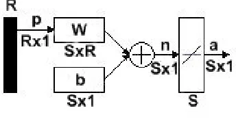
4.1 Introduction to Artificial Neural Networks (ANNs) _____________________ 57 4.2 Notation, Neuron Models and Network Architectures ___________________ 60 4.2.1 Transfer Functions ___________________________________________ 63 4.3 Problem Solving with Different Architectures of ANNs and Learning Rules Used _____________________________________________________________ 67
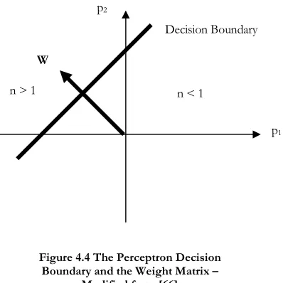
4.3.1 The Perceptron Architecture ___________________________________ 67 4.3.1.1 Perceptron learning Rule __________________________________ 69 4.3.2 The Backpropagation Learning Rule and Architecture_______________ 69 4.3.2.1 The Widrow-Hoff or Least Mean Square Learning Rule _________ 70 4.3.2.2 The Backpropagation Learning Rule and Architecture Used ______ 71 4.3.2 Generalisation of Backpropagation ANNs ________________________ 74 4.3.2.1 Regularisation___________________________________________ 74 4.3.2.2 Pre-processing and Post-processing of Data ___________________ 75 4.4 Conclusion _____________________________________________________ 75
Chapter 5 _________________________________________________ 77
Design of the simulation performed ______________________________ 77 5.1 Choice and Analysis of a Power System ______________________________ 77
5.1.1 Power System Configurations and Contingencies Used in the Voltage Stability Analysis_________________________________________________ 81
5.1.1.1 Contingencies Considered _________________________________ 81 5.1.1.2 How the UWPFLOW Program was Used in the Voltage Stability Studies_______________________________________________________ 82 5.2 The Artificial Neural Networks used for Training ______________________ 83 5.2.1 The Backpropagation ANN Architectures Used ____________________ 83 5.2.1.1 The Selected Backpropagation ANN Architectures _____________ 84 5.3 Conclusion _____________________________________________________ 87
Chapter 6 _________________________________________________ 89
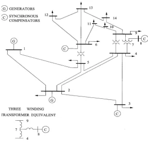
Simulation results _____________________________________________ 89 6.1 Voltage Stability Analysis of the IEEE 14 Bus Test Power System ________ 89
6.2 Training of Backpropagation ANNs and Their Final Errors _____________ 107 6.2.1 Training of Backpropagation ANNs ____________________________ 108
6.2.1.1 The MATLAB Program to Draw Error graphs of the Simulation Results______________________________________________________ 109 6.2.1.2 ANN 1 _______________________________________________ 111 6.2.1.3 ANN 2 _______________________________________________ 112 6.2.1.4 ANN 3 _______________________________________________ 114 6.2.1.5 ANN 4 _______________________________________________ 116 6.2.1.6 ANN 5 _______________________________________________ 118 6.2.1.7 ANN 6 _______________________________________________ 120 6.2.1.8 ANN 7 _______________________________________________ 122 6.2.1.9 ANN 8 _______________________________________________ 124 6.2.1.10 ANN 9 ______________________________________________ 126 6.3 Conclusion ____________________________________________________ 128
Chapter 7 ________________________________________________ 130
Discussion of results __________________________________________ 130 7.1 A Study of the Theory of Voltage Stability___________________________ 130 7.2 Voltage Stability Analysis of the IEEE 14-Bus Test Power System in Full and Under Different Contingencies _______________________________________ 130 7.3 A Study of the Theory of Soft Computing or Artificial Intelligence _______ 133 7.4 Training of Artificial Neural Networks for the Prediction of Voltage Instability in the IEEE 14 Bus Test Power System_________________________________ 133 7.5 Conclusion ____________________________________________________ 137
Chapter 8 ________________________________________________ 139
Conclusions and scope for future work___________________________ 139 8.1 Conclusions ___________________________________________________ 139 8.2 Scope for Future Work___________________________________________ 141
Appendix 1_______________________________________________ 144
Preliminary mathematics ______________________________________ 144 A 1.1 Solution of Scalar Autonomous Differential Equations _______________ 144
A 1.1.1 An Example _____________________________________________ 145 A 1.1.2 Theorem A1.1: The Theorem of Existence and Uniqueness of Solutions
A2.1 Solution of Differential Equations. ________________________________ 158 A2.2 Equilibria and Stability of Equilibria. ______________________________ 161 A2.3 Eigenvectors, Manifolds and Invariance. ___________________________ 164 A2.4 Limit Cycles and the Stability of Limit Cycles. ______________________ 169 A2.5 Bifurcation Theory. ____________________________________________ 172 A1.5.1 Saddle Node Bifurcations. __________________________________ 176 A2.5.2 Hopf Bifurcations. _________________________________________ 181 A2.6 Differential - Algebraic Systems of Equations. ______________________ 183 A2.6.1 Equilibrium Points and Stability in Differential – Algebraic Systems. 184 A2.6.2 Singularity Induced Bifurcations. _____________________________ 186 A2.7 Multiple Time Scale Systems of Differential Equations._______________ 190
Appendix 3_______________________________________________ 191
Appendix 4_______________________________________________ 192
Published papers _____________________________________________ 192 1. Transactions IEEE Pakistan – Accepted for Publication _________________ 192
VOLTAGE INSTABILITY IN POWER SYSTEMS, ITS ANALYSIS AND PREDICTION USING ARTIFICIAL INTELLIGENCE METHODS______ 192 2. Australian Universities Power Engineering Conference 2006 – Published ___ 200 MATHEMATICS OF VOLTAGE INSTABILITY IN POWER SYSTEMS 200 3. Australian Universities Power Engineering Conference 2008 – Published ___ 211
ACKNOWLEDGMENTS
I wish to thank Prof. Akhtar Kalam for his excellent supervision of the research and the writing of the thesis and the help he extended even while on vacation. Thanks are also extended to Victoria University of Technology for giving me the opportunity and the facilities for research.
C h a p t e r 1
INTRODUCTION
Soft computing is a concept that has come into prominence in recent times and its application to power system analysis is still more recent [1]. This thesis explores the application of soft computing techniques in the area of voltage stability of power systems.
Soft computing, as opposed to conventional “hard” computing, is a technique that is tolerant of imprecision, uncertainty, partial truth and approximation. Its methods are based on the working of the human brain and it is commonly known as artificial intelligence. The human brain is capable of arriving at valid conclusions based on incomplete and partial data obtained from prior experience. It is an approximation of this process on a very small scale that is used in soft computing. Some of the important branches of soft computing (SC) are artificial neural networks (ANNs), fuzzy logic (FL), genetic computing (GC) and probabilistic reasoning (PR). The soft computing methods are robust and low cost.
It is to be noted that soft computing methods are used in such diverse fields as missile guidance, robotics, industrial plants, pattern recognition, market prediction, patient diagnosis, logistics and of course power system analysis and prediction. However in all these fields its application is comparatively new and research is being carried out continuously in many universities and research institutions worldwide [2, 3].
and voltage stability, which by itself is a new field. The methods developed in this research would be faster and more economical than presently available methods enabling their use online.
1.1 Problem Statement
In all electrical power engineering courses rotor angle stability is invariably taught as a routine practice. However, while voltage stability has come into prominence in recent times, it is not covered in sufficient depth if at all. Most engineers in the industry are not familiar with the problem and usually confuse it with rotor angle stability or low voltage problems. This is due to the fact that in the past virtually all power systems were designed with ample redundancy and voltage stability was seldom a problem. However, in recent times with reduced investment in power system expansion, load growth particularly in areas with weak transmission and generation and deregulation of the market causing unusual load patterns, voltage stability has come into prominence and theories to explain and analyze it are now being developed [4]. Voltage instability results in voltages in parts of the system or the entire system becoming unstable or collapsing altogether causing collapse of the system. It is also different to low voltages experienced in certain parts of the network during certain conditions, when, though some voltages are low, the system is operating at a stable point. The power system dynamics that take place during voltage instability are non-linear and non-linear analytical techniques, such as Bifurcation Theory are required for its analysis [4].
undergraduate level is the difficulty of the subject coupled with the difficulty of its evaluation. However with the advent of personal computers more and more mathematicians and engineers are paying greater attention to it and computer programs are being written for solution and visualization of solutions, PHASER [14] and MATLAB. There is also a voltage stability specific computer program called UWPFLOW that solves voltage stability specific problems.[15]. Extensive use of this program is made in the present research along with PHASER [14].
A major outage in North America on 14th
August 2003 causing major blackouts in Midwest and Northeast United States and Ontario, Canada has been at least partially due to voltage collapse according to the US-Canada Power System Outage Task Force Report [16].
A recent outage due to voltage instability has also been reported in Sri Lanka [17].
References [18, 19] describe the application of voltage stability theory to analyze the South-Brazilian and Ecuadorian Power Systems and how the results thus obtained agreed with operational experience where voltage collapse has been experienced before. Thus voltage stability is not merely a theoretical construct but reality for which there was no urgency till recent times when power systems became more and more stressed due to aforementioned reasons.
1.2 Aim
The aims of the research reported in this thesis are as follows.
• To make a thorough study of the theory of voltage stability (instability).
• To study the methods of soft computing in general and Artificial Neural Networks in particular.
• Analyze the IEEE 14-bus system under different contingencies to obtain proximity to voltage collapse indices. The analysis will be performed using the UWPFLOW computer program.
• To use the results of the computer analysis to develop artificial neural networks (ANN’s) suitable for the prediction of pending voltage instability in power systems thus developing a soft computing method of power system security assessment. This is the main aim of this research. Though the implementation is not a part of this project, ANN’s developed will be suitable for on-line use in real power systems. For this purpose the ANN’s need to be embedded and trained in dedicated hardware with inputs of the suitable power system parameters which will be identified.
• To relate the results to the hypothesis (Section 1.3).
• To identify topics suitable for further research on the subject.
1.3 Hypothesis
After reading the available literature on voltage stability and soft computing methods the following hypothesis was formed.
1.4 The Research Method
The following approach which includes the method used to obtain results was used in the research.
• The relevant mathematics was studied in detail. Refer to appendices 1 & 2.
• A study was made of the theory of voltage stability/instability. Although a highly technical textbook [4], is available and is very good for the understanding of voltage stability phenomena, other sources such as journal papers and the IEEE/PES Special Publication on Voltage Stability [20], were found to be more useful in the actual research method implemented during the voltage stability computer simulations. The computer program used is UWPFLOW [15].
• Data on voltage stability for the IEEE 14-bus test system was generated using UWPFLOW to be used to train the ANN’s and illustrate the phenomenon of voltage instability in power systems.
• Artificial Neural Network theory was studied and ANN’s for the prediction of voltage instability in power systems were trained and tested.
1.5 A survey of the available literature on voltage stability in power systems
As stated before voltage stability/instability has come in to prominence or has even been recognised only in comparatively recent times. Therefore the available literature on the topic is still tentative and often repetitive. Two recent attempts at formalising the theory and facilitating its analysis are presented in References [4, 20].
Placing the voltage stability problem in context, the references [16-19] describe real life voltage stability problems, some of which caused major outages in North America, Sri Lanka, Brazil and Ecuador.
The IEEE journal article [21] giving definitions and classifications of power system stability recognises voltage stability and gives a brief description and definition.
The References [22-25] are good examples of the original efforts to develop and consolidate a dynamical systems based theory of power system stability in general and voltage stability in particular. These are initial efforts and a theory of voltage stability is only beginning to take shape.
Later a series of papers some of which are given in references [35, 36, 38, 40-50], were published that considered different methods of calculating the voltage stability of power systems. Broadly the methods fall in to two categories, direct methods and continuation methods. The different papers vary mostly only in the detail of the methods rather than the mathematical principles involved. The point of collapse and continuation power flow methods put forward in reference [35] are the methods used in the computer program UWPFLOW; both the paper and the computer program are by the same author. This computer program is the only reasonable program that is available to researchers without spending too much on purchase of the software.
Modelling of power system components such as generators, lines, loads, etc. are presented in references [4, 20, 36, 38, 43, 45, 51].
Indices for the prediction of proximity to voltage instability are presented in references [4, 20, 37, 39, 52, 53] and compared.
A mathematical function called a Lyapunov Function is used in the analysis of dynamical systems. In voltage stability analysis this function is called an Energy Function and its derivation is put forward in references [20, 24, 54-61]. Using this energy function proximity to voltage instability can be calculated as an index.
1.6 Originality of the Thesis
The thesis contains original work of the author except where reference is made to published literature. The choice of parameters for the training of ANN’s and the particular ANN architectures chosen are new in the field of voltage stability prediction as far as the author has been able to ascertain after an extensive search of the available literature. Therefore the thesis would be an original contribution to and an expansion of the present knowledge in the field of voltage stability in general and the application of soft computing or artificial intelligence to voltage stability estimation in particular.
1.7 Thesis Organisation
Chapter 1 - Introduction
This Chapter introduces the intent of the thesis. The problem of voltage stability in power systems which has recently come into prominence is briefly explained. An aim and a hypothesis for the thesis are formulated and the research method appropriate for the stated aim of the research is formulated. Section 1.5 gives a survey of the available literature on the subject. A statement of originality of the thesis is given in Section 1.6.
Chapter 2 – Voltage Stability
somewhat recent too and it is difficult to come to grips with the subject without reading a large number of them.
Chapter 3 – Methods for Evaluation of Voltage Stability in Power Systems and Indices Used to Measure Proximity to Voltage Instability This Chapter explains methods used to evaluate the voltage stability of power systems off line and the various indices proposed in the literature to measure proximity to voltage instability in power systems with their relative merits. The methods used in this thesis will be indicated.
Chapter 4 – Soft Computing or Artificial Intelligence Methods – Brief Theory and Selection
A brief theory of soft computing or artificial intelligence methods is introduced in this Chapter. Reasons for the selection of artificial neural networks in general and the types of neural networks used in particular are explained.
Chapter 5 – Design of the Simulation Performed
This Chapter explains the design of the power system simulations performed for the evaluation of voltage stability in the IEEE 14-bus test system and its variations selected by the author of the thesis. The reasons for the particular design used are explained. The design and training of the ANN’s used is also explained.
Chapter 6 – Simulation Results
Chapter 7 – Discussion of Results
A discussion of the results in the context of the aims of the research undertaken is given in this Chapter. Section 1.2 presents the aims in point form and a summary of these aims is used as the relevant section headings in this Chapter.
Chapter 8 – Conclusions and Scope for Future Work
Finally the conclusions of the research with respect to the hypothesis presented in Section 1.3 are presented here. The discussion of the results with respect to the aims of the research is presented in Chapter 7. Topics for further related research are also identified.
1.7.9 Appendices 1 & 2
C h a p t e r 2
VOLTAGE STABILITY
2.1 Introduction
In the past adequate redundancy was built into power systems for voltage instability to be a major problem. Only rotor angle stability was considered in the operation and expansion of power systems. With the introduction of the new electricity market resulting in reduced investment and altered load patterns, particularly increasing load in areas with weak transmission and generation capacity, voltage stability has come into prominence [4, 20]. Voltage stability requires mathematical theory and concepts that are difficult to understand.
2.2 Some Useful Definitions.
The following two definitions of stability of a power system are given in [20].
1. An operating point of a power system is small disturbance stable if, following any small disturbance, the power system state returns to be identical or
close to the pre-disturbance operating point.
2. An equilibrium of a power system model is asymptotically stable if, following any small disturbance, the power system state tends to the equilibrium.
The second definition assumes that the power system is modelled by a set of differential equations.
Voltage instability stems from the attempt of load dynamics to restore power consumption beyond the capacity of the combined transmission and generation
system.
2.3 Voltage Instability
A power system operating under stable conditions keeps continuously evolving. During this process some or all of the following take place in the system. The load changes; generators and induction motors go through electromechanical transients; static VAR compensators, (SVCs), activate; on load tap changers in transformers activate; shunt capacitors are switched on and off; automatic load recovery takes place following faults; faulted components of the power system are isolated; faulted transmission and distribution lines auto-reclose; excitation limiters activate etc. Thus a power system under load is a dynamical system. During this dynamics, if the power system is to remain stable, the operating point or the equilibrium point of the system has to track a stable point in state space. However, the transmission system has a limited capacity for power transmission and generators have a limited generating capacity, on reaching these limits the system can go into voltage instability. At the point of going into voltage instability, the stable point of operation that existed before disappears. Thus the power system undergoes a transient and during this transient, the voltages decline causing a voltage collapse. It is to be noted that the state of a power system operating with low voltages but at a stable point, i.e. there is no dynamic collapse of the voltages, does not constitute a voltage stability problem.
2.4 Voltage Instability in an Elementary DC Power System
Consider a simple dc power system fed by a dc power source of 1V. The line resistance is 0.5Ω, the load is a variable resistor and I is the current drawn by the load.
E=1V V
R=0.5Ω
RL
Figure 2.1 An Elementary dc Power System
The load resistance RL is automatically varied to achieve an assumed
maximum power demand of 0.55W according to the differential equation:
(2.1)
According to elementary circuit theory, the maximum transferable power Pmax
is given by:
(2.2)
However in this example a power demand of 0.55W is placed on the system.
The trajectory of the load resistance given by the solution of the differential equation (2.1) with an initial condition of RL =4.5Ω is shown in Figure 2.2.
2
0.55
L L
R =I R −
2
max 0.50
4 E
P W
R
Figure 2.2 Trajectory of the Load Resistance
The variation of the load voltage and load power as the system power demand increases are shown in Figures 2.3 & 2.4.
P
(
W
)
t (s)
Figure 2.4 Variation of Load Power
It is seen from Figures 2.3 & 2.4 that voltage instability or collapse takes place when the demand for power increases beyond the maximum deliverable power of 0.5 W. Obviously the dynamics obtained in an actual power system is far more complicated.
The dynamics of a loaded power system, as the dynamics of many other systems in engineering, can be represented by a system of non-linear ordinary differential equations, which can be written as:
( )
x= f x (2.3)
where usually x dx dt =
where t is time, x is a (n×1) vector and , ( 1, 2,.... )
i
f i= n are generally non-linear functions of xi, (i=1, 2,.... )n . The vector x represents the state of the system at a given time and is known as the state vector. Systems of this type are known as dynamical systems.
geometric theory of ordinary differential equations allows the study of the behaviour of dynamical systems without resort to integration. [5-13].
2.5 Classification of Power System Stability
Table 2.1 shows a convenient classification of power system stability. It is similar to Table 1.1 in reference [4] but has been modified for better clarity of understanding.
Table 2.1 Classification of Power System Stability
Time Scale
General Description -
generator driven Generator driven Load Driven
Short Term
Steady state or small signal stability. Transient or large disturbance stability Rotor angle stability both transient and steady state Short term voltage stability Long Term Insufficient generation Frequency stability Long term voltage stability
no strict distinction is made between long term and short term voltage stability. [4].
The dynamic nature of a power system was touched upon in Section 2.3. The dynamics mentioned there take place in the general time scales given in table 2.1. A further elaboration of the time scales in which voltage instability may take place is as follows.
1. The time scale of electromechanical transients such as those of generators, regulators, induction machines and power electronics (eg. SVC’s), takes place in the range of seconds.
2. The time scale of discrete switching devices such as on load tap changers and excitation limiters, takes place in the range of tens of seconds.
3. The time scale of load recovery processes, takes place in the range of several minutes or even hours.
The time scale 1 as aforementioned is the short term or transient time scale in voltage stability while the time scales 2 & 3 are the long term time scales. Electromagnetic transients such as dc components of short circuit currents take place in too short a time scale to be of any relevance in voltage stability and therefore are not considered. It should also be noted that a voltage collapse that starts in the long term time scale could end up as a transient or short term collapse. That is initially the voltages in the power system collapse slowly but towards the end of this collapse the rate of collapse accelerates causing a catastrophic failure of the power system. [20].
and loads while the focus of classical transient stability is generators and angles.
2.6 Theory of Voltage Stability
As mentioned earlier in the thesis, a power system is a nonlinear dynamical system and in the analysis of voltage stability, mathematics of dynamical systems is used. Though in the past, engineers have from time to time used the methods of dynamical systems for problem solving, it has remained mainly the province of mathematicians due to its difficulty. Even among mathematicians not many have devoted much time to it due to its computational difficulties and the need to grasp and visualise its concepts in many dimensions. However with the advent of personal computers easing the computational burden, more and more authors are paying attention to it. Some of the available books on the subject are [6-13]. There is a computer program ‘PHASER’ [14] specifically designed for evaluation and visualisation of the behaviour of dynamical systems. The author of this thesis used this program to solve some of the specifically designed problems which are presented in Appendix 1. Appendices 1 & 2 present the mathematics of dynamical systems and will be referred to in the rest of this section along with other references. It should be emphasised that dynamical systems are solved, given the initial conditions, using qualitative or geometric theory of ordinary differential equations rather than analytical methods. These systems are very difficult or impossible to analyse analytically.
2.6.1 A Brief Description of Relevant Mathematics
A dynamical system is usually represented by a set of n differential equations as follows: (Refer to Appendices 1 & 2, particularly appendix 2 for detailed explanations and references.)
Here x is a (n x 1) vector, f x( ) is a set of (n) nonlinear functions of x and x is the time differential ofx. Given the initial conditions and under certain conditions the system can be solved to give a trajectory of the system over time in the n-dimensional space ofx. These trajectories have intervals of existence that may be finite or infinite.
Equilibrium points are particular solutions of the equation (2.1) where the solutions stay at these equilibrium points for all time. Equilibrium points are given by the solutions to the following equation:
f x( )=0 (2.2)
An equilibrium point may be unstable, stable or asymptotically stable with a region of attraction.
If equation (2.1) represents a nonlinear system then the following apply.
• The number of equilibria of the system may be one, more than one or none.
• The existence of a stable equilibrium is not a guarantee of the stability of the system since the region of attraction of the stable equilibrium may be limited.
The stability of an equilibrium point of a nonlinear system of the type shown in equation (2.1) may be determined by linearising the system around the equilibrium point and obtaining its Jacobian.
• If at least one eigenvalue of the Jacobian has a positive real part, then that particular equilibrium point is unstable.
2.6.1.1 Bifurcations
The instabilities of interest in power system voltage stability are bifurcations.
Consider a dynamical system of the following form.
x= f x p( , ) (2.3)
where x is a (n x 1) state vector and p is a (k x 1) parameter vector. For every value ofp, the equilibrium points of the system are given by:
f x p( , )=0 (2.4)
These equilibrium points fall on a k-dimensional manifold in the (n + k)-dimensional space of state and parameter vectors. At a bifurcation point for the given value ofp , the Jacobian of equation (2.3) with respect to x is singular. A saddle node bifurcation (SNB) is a bifurcation where two branches of equilibria meet. (Refer to Appendix 2.) So at a saddle node bifurcation two equilibria coalesce and disappear. One of the equilibria has a real positive eigenvalue and the other has a real negative eigenvalue. Both become zero at the SNB.
At a Hopf bifurcation a pair of complex eigenvalues crosses the imaginary axis and causes an oscillatory instability.
2.6.1.2 Differential Algebraic Systems
Some dynamic systems are represented by a set of differential equations with algebraic variables where these algebraic variables are subject to a set of algebraic constraints represented by a set of algebraic equations as follows:
0=g x y p( , , ) (2.5b)
where x and pare as in equation (2.3) and yis a (m x 1) vector of algebraic variables. The algebraic equation (2.5b) defines a (n + k)-dimension constraint manifold which is a hypersurface where the solutions to the system occur.
At singular points of the m algebraic equations, ie. when the algebraic Jacobian is singular, the response of the system is undefined and causes singularity induced bifurcations.
When the algebraic Jacobian is non-singular, the response of the system can be studied by studying the reduced Jacobian of the system given by equation (2.5). This will give the bifurcation points and other relevant data of the system.
2.6.1.3 Singular perturbation or Time Scale Decomposition
Some systems, including power systems, have dynamics evolving in different time scales. That is these systems have dynamics evolving in slow and fast time scales. Such systems are represented as follows.
x= f x y( , ) (2.6a)
εy=g x y( , ) (2.6b)
where x is a vector of slow states, y is a vector of fast states and
ε
is a small number.In singular perturbation or time scale decomposition, the method used to study such systems, it is assumed that ε →0. Then the system reduces to a differential algebraic system as follows:
0=g x y( ,s s) (2.6d)
This system contains only slow state variables and can be studied by the methods used for differential algebraic systems. It is assumed in the analysis that the fast dynamics is stable and that it has died out.
2.7 Application of the Theory to Power Systems
In equation 2.3 reference is made to two types of variables in a dynamical system namely states and parameters. In a power system, which as stated above is a dynamical system, examples of states are bus voltage magnitudes, bus voltage angles, machine angles and currents in generator windings. Examples of parameters are real power demands at system buses and sometimes control settings that determine how different power system and generator controls behave. [4, 18-20, 26-29, 31, 32, 35, 36, 40, 41, 44]. The choice of states and parameters used in a particular study of voltage stability is dependent on the method of analysis chosen in that instance. Refer to Chapter 3 for the method of study used in this thesis.
to be noted that both system states and parameters are vectors and therefore the state space and parameter space of a power system are multi-dimensional consisting of hundreds and sometimes thousands of dimensions each. Therefore the following explanation is confined to 1, 2 or 3 dimensions. Higher dimensional problems can be calculated and manipulated mathematically, (refer to Appendices 1 and 2), though they are impossible to visualise.
2.7.1 A Simple Power System
Consider the simple power system shown in Figure 2.5.
Figure 2.5 A Simple Power System
The figure shows a single PV or constant voltage or slack bus with a single generator connected to it supplying a constant power factor PQ load consisting of real and reactive parts equal to p(1+jk).
Let the impedance of the line be (0+ jX) as resistance is neglected. Then, if I is the line current and (S = p+ jq)is the load power, it can be shown that [4, 20]:
V =E− jXI (2.7)
PV
E,0o
V,δo
jX
PQ
(2.8 a and b)
The above equations are written on the assumption of quasi-steady-state in which case they reduce to power flow equations. More will be discussed on this topic in Chapter 3.
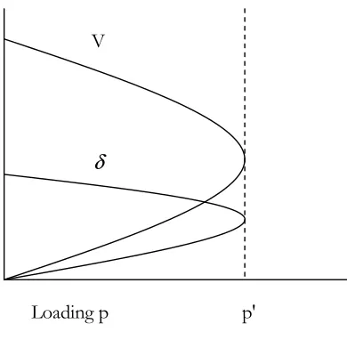
Now, if real power p is chosen as the slowly varying parameter and V and δ are chosen as the state vector, the variation of the magnitude of V with p is as shown in Figure 2.6. Such a diagram where one of the state variables is plotted against the slowly varying parameter, p in this case, is called a bifurcation diagram.
Figure 2.6 Bifurcation Diagram of State V Vs Parameter p
It is seen from the bifurcation diagram that for loads less than p' there are two V
Loading p p'
2
2
( cos sin )
sin
cos j
S EV jEV V
voltage and high current. In practice the high voltage equilibrium is the more stable and the equilibrium at which a power system operates. As the slowly varying parameter, power p, is increased at the load bus, the two equilibria come closer and coalesce at the critical power p' which is a saddle node bifurcation. Beyond p' the power system has no equilibrium points and cannot be operated. At p' voltage collapse occurs.
In Figure 2.7 both power system states V and δ are plotted against p.
Figure 2.7 Bifurcation Diagram of States V & δ Vs Parameter p
In this diagram the lower value of angle δ refers to the stable higher value of voltage V. It is seen that the noses of both curves representing a saddle node bifurcation occur at the same critical loading p'.
The occurrence of voltage stability and instability can also be visualised in state space as follows: (It is to be emphasised that the Figures 2.6 and 2.7 are bifurcation diagrams). Figure 2.8 shows the case of the above simple power system operating at a stable equilibrium where the load power is less than p'.
Loading p p'
V
Figure 2.8 State Space at Loads Below Critical Loading p'
It is seen that any small perturbation from the upper equilibrium at the higher voltage causes system dynamics that bring the operating point back to the equilibrium. The diagram also shows that the low voltage equilibrium is unstable. Any small perturbation from this equilibrium invariably causes a catastrophic collapse of the power system unable to reach an equilibrium.
Figure 2.9 shows state space at the critical loading of p'. V
Figure 2.9 State Space at Critical Loading p'
At this loading the two equilibria have coalesced into one equilibrium. Any small perturbation from this equilibrium will cause power system states to move in the direction of the thick arrow casing a monotonic decrease in the system voltage and an increase in the angle δ. This is the mechanism of voltage collapse in a power system.
Figure 2.10 shows the state space of the simple power system above subsequent to voltage collapse at a saddle node bifurcation.
V
Figure 2.10 State Space Subsequent to Voltage Collapse at a Saddle Node
Bifurcation
The voltages fall monotonically unable to find an equilibrium.
In a real power system the state space would be, as aforementioned, multidimensional consisting of hundreds if not thousands of states.
2.7.1.1 A Two Load Power System in Parameter Space
Figures 2.8 to 2.9 showed a single load power system in state space. Similarly a power system can also be visualised in parameter space for voltage stability studies. To do so at least two load buses need to be considered. Let the real power loads at the two buses be p1 & p2.
Referring to Figure 2.11: V
Figure 2.11 Parameter Space of a Two Load Bus Power System
In the region marked ‘Stable Region’ there are stable equilibrium points where the power system may be operated stably with any combination of p1 & p2 that falls in that region. However in the region marked ‘Unstable Region’ the power system has no equilibrium points at which it can operate stably and any loading that reaches this region will cause voltage collapse. In the figure loading point p is stable, however if the power system is stressed by increasing the load in the direction of the arrow it will reach the point p' which is a saddle node bifurcation and voltage collapse will ensue. Thus the power system always needs to be operated in the stable region. The two regions are separated by a curve called the bifurcation set. The bifurcation set for a power system with n real power loads (parameters) is a hyper surface of (n-1) dimensions and the parameter space is n-dimensional.
2.7.1.2 Voltage Instability Caused by a Large Disturbance
Voltage instability may result in a power system that undergoes a large disturbance such as the loss of a transmission line or a generator due to a
Unstable Region
Stable Region p
P'
Load p1 at Bus 1
L
o
ad
p
2
at
B
us
fault. Before the disturbance the power system is operating at a stable equilibrium, however, after the disturbance that causes the loss of a major component, the power system may be left without a stable operating point or equilibrium. This would cause a catastrophic collapse of the system voltages. In state space this is the equivalent of the power system abruptly going from the state represented in Figure 2.8 to the state represented in Figure 2.10 without first reaching the saddle node bifurcation represented in Figure 2.9. In parameter space this can be represented as the system, operating stably, as represented by the point p in Figure 2.11 and then immediately after the disturbance finding itself operating in the unstable region as shown in Figure 2.12.
Figure 2.12 Parameter Space of a Two Load Bus Power System Operating at an
Unstable Point
In Figure 2.12, the operating point p of the power system has not moved but the stable operating region of the power system has shrunk due to the disturbance and now the operating point is outside the new modified stable
Unstable Region
Stable Region p
Bus 1 Load p1
B
us
2
L
o
ad
p
2.7.1.3 Voltage Instability Caused by Power System Limits
During the operation of a power system various limits are invariably encountered. Examples of these limits are generators reaching their reactive power limits and on load tap changing transformers reaching the limits of the tap ranges. Consider a generator with reactive power limits and the nose curves of the power system drawn for a particular bus with the bus voltage on the y-axis and the system real power drawn on the x-axis. When so drawn, the nose curves are also bifurcation diagrams and are shown in the following Figures 2.13 and 2.14. The upper portions of the nose curves represent the stable equilibria of the power system.
Figure 2.13 Equilibrium Point B Remains Stable On Reaching Reactive Power Limit
V
Loading p
Limit Off
Limit On A
Figure 2.14 Equilibrium Point B Becomes Unstable On Reaching Reactive Power
Limit
In both figures consider the system starting operation at point A. Point A is not a zero power point since the x-axis starts at a value greater than zero, the base condition of the power flow study. At this point in time, the generator reactive power limit is off, that is the generator is capable of supplying more reactive power. As the parameter p (system real power) increases, the system equilibrium or operating point moves along the ‘limit off’ nose curve. Now if it is assumed that the generator reaches its reactive power limit at point B, then the nose curve which is also the bifurcation diagram changes to the ‘limit on’ nose curve. In Figure 2.13 it is seen that the point B falls on the stable part of the ‘limit on’ nose curve and therefore the power system continues to function in a stable state though with a smaller margin to voltage collapse. However if the ‘limit on’ nose curve of the system is as shown in Figure 2.14, then the power system operating point is on the unstable part of the new nose curve and therefore the system collapses at a limit induced bifurcation.
V
Loading p
Limit Off
Limit On
A
2.7.1.4 Voltage Stability in a System with Both Slow and Fast Time Scales
Equations 2.6c and 2.6d represent the time scale decomposition of a system with both slow and fast time scales. In the two equations it is assumed that the fast transients are stable and that they have died out. Such a system with only one slow variable x and one fast variable y is represented in Figure 2.15 in the x-y plane.
Figure 2.15 A System with Slow and Fast Time Scales
The curve g=0 is the fast dynamics equilibrium manifold, that is, on this manifold fast dynamics do not take place. Only the slow components of y and x vary on this curve. That is, this is a good approximation of the slow manifold of the two time scale system. Now the equilibria of the complete system with both slow and fast components are the intersection of the curves g=0 and f=0. The upper equilibrium is stable and the lower equilibrium is unstable. The arrows in the diagram indicate the direction of movement of the system operating point for any initial condition. As an example, if the initial condition of the system is at A in the figure, then a fast transient takes
y (fast)
x (slow) A
f=0
g=0
Equilibriums Stable
place that brings the operating point to the upper stable part of the fast dynamics equilibrium manifold and then moves slowly along this slow manifold of the two time scale system till the stable upper equilibrium of the two time scale system is reached and continues to operate there. In an actual power system obviously there will be many variables x and y and therefore Figure 2.15 would be multi-dimensional.
In a two time scale system it can also happen that the curves g=0 and f=0 do not intersect. For example the curve f=0 may be some distance removed from the curve g=0 in the positive direction along the x-axis. If the power system has reached such a state then a saddle node bifurcation of the fast dynamics can take place since the two curves or manifolds do not intersect at system equilibria. In this case, for an initial condition at A, the system again is brought to the fast dynamics equilibrium manifold through a fast transient and starts moving along this manifold in search of a system equilibrium. But since no system equilibrium exists, the operating point reaches the nose of the fast dynamics equilibrium manifold which is a saddle node bifurcation of the fast dynamics causing voltage collapse.
2.8 Conclusion
C h a p t e r 3
METHODS FOR EVALUATION OF VOLTAGE STABILITY IN POWER SYSTEMS AND INDICES USED TO MEASURE
PROXIMITY TO VOLTAGE INSTABILITY
There are a number of methods of evaluating voltage stability in a power system. However the method chosen in a particular case depends on the resources available, time constraints and the required depth of analysis. Since voltage stability is still a developing field one has to be rather cautious in the method and resources used. The program used for this thesis is UWPFLOW [15]. This chapter, as the title suggests, will examine the methods of evaluation of voltage stability in a power system and indices used to measure proximity to voltage instability in a power system with emphasis on the method used in the thesis.
3.1 Background
Until now time power system engineers have used power flow programs and transient angle stability programs in the analysis of power systems during design and operation [4, 20]. However, due to reasons mentioned in Section 2.1, it has now become necessary to consider voltage stability as well.
Power flow programs use static analysis using algebraic equations to obtain the condition of the power system at a particular point in time. This point in time may be after the active and reactive powers have changed in some or all of the buses or the system configuration has changed due operational reasons or fault conditions.
components such as synchronous machines, excitation systems, turbines and their governors, static var compensators (SVC’s), high voltage direct current transmission, loads etc. These models are suitable for analysis in the time frame of a few milliseconds to a few tens of seconds.
However voltage instability can develop in the time frame of up to many tens of minutes, references [4, 16, 20, 64]. Thus a careful choice of the method depending on resources and time available is needed in the analysis of voltage stability.
3.2 Methods Used in the Analysis of Voltage Stability
Voltage security of a power system in the context of its general security is explained very clearly in reference [4] which is summarised below.
A power system is subjected to two types of constraints:
• Load constraints state that the load demand is met by the system and are expressed as equality constraints.
• Operating constraints impose maximum and minimum limits on variables such as line currents, bus voltages, generator real and reactive power etc. These are expressed as inequality constraints.
When both load and operating constraints are satisfied the power system is in a normal state. On the occurrence of a disturbance the system may settle down to a new normal state or one of two abnormal states. An emergency state is an abnormal state when some operating constraints are not satisfied. A restorative state is an abnormal state when operating constraints are satisfied but some or all the load constraints are not, due to say a partial blackout or load shedding.
dynamic emergency occurs when a disturbance causes the system to become unstable due to say loss of synchronism. Static security assessment deals with the ability of the system not to enter a static emergency after a disturbance. Dynamic security assessment deals with the ability of the system to reach a stable operating point after a disturbance and is a prerequisite for system security.
Corrective control or corrective operator action is often possible in a static emergency but a dynamic emergency requires action by automatic devices.
Voltage stability belongs to the category of dynamic emergencies where a stable operating point is lost requiring automated action, however if a pending voltage instability could be predicted sufficiently in advance then corrective operator action may be possible. This is still beyond the state-of-the-art, reference [4], and the research presented in this thesis is an attempt at rectifying this.
In voltage security analysis, a power system is evaluated for voltage stability during credible contingencies such as the loss of transmission and generation facilities. The general rule adopted is the well-known (N-1) criterion where a power system is expected to perform without entering an emergency state for contingencies when a single transmission line or a single generator trips out. [4].
As will be seen below in this Chapter static analysis tools can be used for voltage security analysis and often is the main tool used. However this should not detract from the fact that voltage instability is a dynamic problem.
3.2.1 Dynamic or Time Domain Analysis.
• Synchronous machines.
• Excitation systems.
• Turbines.
• Governors.
• Loads.
• High Voltage Direct Current (HVDC) transmission equipment.
• Static Var Compensators (SVC).
post-3.2.2 Quasi Steady State (QSS) Method or Analysis
The quasi steady state method makes use of the method known as singular perturbation or time scale decomposition presented in Sections 2.6.1.3, 2.7.1.4 and A2.7.
In this method the fast dynamics of fast responding components of the power system are neglected and represented by their equilibrium equations. The long term dynamics of components such as shunt compensation, on load tap changers, secondary voltage and frequency controllers, loads etc are represented by differential or difference equations. The algorithm uses suitable time steps and at each time step (call this the present time step) calculates the values of the states assuming that the slow dynamics remains static at the value at the end of the previous time step. Then these new state values are used in the equations for slow dynamics to calculate corrected values for states at the present time step. The calculations are repeated at each time step for the required period of time [4].
The quasi steady state method has been found to be about three orders of magnitude faster than the complete time simulation by dynamic analysis [20]. Therefore it is suitable for studies of large power systems with numerous possible network and equipment configurations.
3.2.3 Use of Traditional Power Flow Analysis
analyses can be performed with suitable increments of real power demand till an unstable operating point is reached [4, 20]. However there are a number of drawbacks to this method. A number of modelling assumptions are made in traditional power flow analysis programs, some of which are as follows [20]:
1. The real power dispatch of generators are fixed with a swing bus to handle the slack.
2. Loads are assumed to be constant P and constant Q without voltage and frequency sensitivity.
3. On load tap changer action is assumed to be instantaneous.
4. Capacitors and reactors are assumed to be either fixed to the network or switched instantaneously.
5. Generator limits are represented as maximum and minimum reactive power limits.
6. PV buses are assumed to have perfect voltage control.
The algorithms used in power flow programs tend to be unstable and non convergent as an unstable operating point is approached due to the Jacobian of the power flow equations tending to zero. Therefore it is not possible to know definitely when an unstable point is reached since the lack of a solution to the power flow equations could be due to limitations of the solution algorithm as the bifurcation point is neared rather than on reaching the bifurcation or unstable operating point.
3.2.4 Energy or Lyapunov Function Analysis
In the theory of dynamical systems and control theory, Lyapunov functions, which are a family of functions that can be used to demonstrate the stability of some state points of a system, are used as one of the methods of analysis. In voltage stability analysis these functions are called energy functions since they have not been proved to be true Lyapunov functions. References [20, 54-61] deal with the topic. This method of analysis has not been used in this thesis since suitable computer programs are not yet available to analyse systems of suitable size for a thesis and also since the methods used in this thesis give more accurate results.
3.3 Power System Component Modelling for Voltage Stability Studies As mentioned in Section 3.2.1 voltage stability takes place in the time scale of one or two orders of magnitude greater than that of transient stability. Therefore component models used in traditional transient stability or standard power flow analysis are inadequate for voltage stability analysis. This section describes briefly some of the methods used in voltage stability programs to take into account the behaviour of various components over the long periods of time studied in voltage stability. References [4, 20, 51, 65-67] deal with this subject in greater detail.
Ideally all components of a power system need to be modelled accurately; however, the type of data available, the limitations of the models available and the practicalities of keeping the system manageable so that the number of equations that need to be solved is kept to a minimum require some system reduction. Due to the very nature of voltage stability that makes it dependent on reactive power demand and supply it is necessary to represent these variables accurately though [4, 20].
transient stability analysis these effects are often neglected. As the voltage drops, loads exhibit a thermostatic effect whereby the energy consumed drops. As a result these loads tend to remain active for a longer time for example to bring the temperature to the set point. Therefore after a period of time within the voltage collapse time frame, the average load returns to the original value thus exacerbating any voltage stability problems.
In addition to the thermostatic effect, OLTC transformers and other voltage restoration devices between the transmission system and the loads on the distribution system act to restore the load voltages during a voltage collapse scenario again exacerbating the problem by restoring the loads to nominal values.
3.3.1 Load Modelling
Load modelling for voltage stability studies and the study of other power system phenomena is still an ongoing project and a number of papers [19, 65-67], have been published. As mentioned above [4, 20] also deal with the subject. The model used in this thesis is based on the polynomial load model mentioned in these references which can be accommodated in the UWPFLOW program used by the author. The model is presented briefly below and the reader is referred to the above references for details.
In the polynomial model used in this thesis the load at a given bus is divided into two parts, a constant impedance part and the balance, usually a constant current part. The effective load at a given voltage is calculated as follows:
Let,
Pl = Effective real power load at per unit voltage V of the bus,
Ql = Effective reactive power load at per unit voltage V of the bus,
Qz = Constant impedance part of the reactive power at the bus,
Pn = Balance real power at the bus,
Qn = Balance reactive power at the bus,
a and b are given constants relevant to the load under consideration.
Then,
. a . 2
Pl=Pn V +Pz V (3.1a)
Ql=Qn V. b+Qz V. 2
(3.1b)
If a = b= 1, then Pn and Qn are constant current parts of the given load.
It is assumed that Equations 3.1a & b take into account the effects of tap changers and other voltage control devices in the distribution network.
3.3.2 Generator Modelling
Generator modelling suitable for voltage stability is an important aspect of detailed voltage collapse studies. References [4, 20, 51] deal with the subject in some detail.
The desired models are those for generator capability curves and over excitation limiters. The above references deal with the subject.
intelligence methods can be used to predict voltage instability in power systems, this is considered not to be a drawback. It is only a compromise in the details and with more sophisticated tools of analysis it can easily be overcome without compromising the conclusions drawn in this thesis.
3.4 Indices Used to Measure Proximity to Voltage Collapse
In voltage stability analysis it is useful to know, given a particular operating point of the power system, how far this operating point is to voltage instability. This enables the operators to anticipate and take precautionary measures to avoid any pending voltage instability. In fact the aim of this thesis is to develop an artificial intelligence method to predict the distance to voltage stability of a power system from any stable operating point.
A number of voltage stability indices have been proposed in the literature [4, 20, 26, 32-51, 53, 55, 63]. Many of these papers are repetitions in some form or slightly improved versions of a given method. Some of the methods have taken hold in the research community and some have not. Discussed briefly below, avoiding mathematical detail, are some of the more relevant indices and methods. The reader is referred to the above references particularly [4, 20] for details.
3.4.1 Loading Margin
The loading margin to voltage collapse is defined in the above references as the change in loading between the operating point and the loading at point of voltage collapse. Considering Figure 2.6, the nose curve for a power system, the loading margin is the difference in loading between any stable operating point on the upper part of the nose curve and the tip of the same curve.
The following advantages of the load margin index to voltage collapse are given in [20]:
• The loading margin is straight forward, well accepted and easily understood.
• The loading margin is not based on a particular system model; it only requires a static power system model. It can be used with dynamic models, but it does not depend on the details of the dynamics.
• The loading margin is an accurate index that takes full account of the power system nonlinearity and limits such as reactive power control limits encountered as the loading is increased. Limits are not directly reflected as sudden changes on the loading margin.
• The loading margin accounts for the pattern of load increase.
3.4.1.1 Continuation Method of Determining Loading Margin Using Nose Curves
Figure 3.1 Continuation Method – Modified from Reference [1]
Since it is the long term voltage stability that is of interest in voltage stability studies, a stable operating point of the power system is obtained by the following equilibrium version of the power system equations given in [4]:
F z p( , )=0 (3.2)
Where z represents the states of the system and p is the varying parameter of interest. In the case of a power flow study, which is of interest here, z represents the vectors of bus voltages and angles and p represents varying system power.
If standard power flow methods are used, as the system approaches the bifurcation point at the nose of the nose curve, the equations exhibit convergence difficulties. Also a large number of different power flow studies with small increments of system power are computer resource and time consuming. These difficulties are overcome as described below.
V
Loading p p'
The continuation method uses a predictor corrector method of drawing the nose curve for a given bus, Figure 3.1. The references [4, 20, 26, 32, 35, 36, 38, 40-45, 47, 53] deal with the subject in detail and give the mathematical theory behind the method. The method starts with a known stable operating point obtained after performing a standard power flow. From this known stable point, the method proceeds as shown in Figure 3.1 by increasing the varying parameter p in small steps and calculating predicted and corrected points on the nose curve. The white dots represent the predicted values and the black dots represent the corrected values. Suitable numerical methods are used to obtain the predicted and corrected values; refer to the above references. However there is a drawback in this method in that as the nose of the curve, which is the bifurcation point, is approached the numerical method tends not to converge as indicated by point A in Figure 3.1. To overcome this, as the nose is approached, the increment in the varying parameter p, is decreased.
3.4.1.2 Continuation Method with Parameterisation
3.4.1.3 Direct or the Point of Collapse Method
Considering Equation 3.2, the bifurcation point, which is the nose of the nose curve and therefore the loadability limit, may be obtained by solving the following set of equations:
( , ) 0 0
1
z
F z p
F v v ∞ = = = (3.3) where,
Fz = Jacobian of Equation 3.2 with respect to z, the states
v = the right eigen vector
||v||∞ = mathematical L∞ norm of v.
In Equation 3.3, the first equation is the equilibrium condition of the power system, the second equation is the singularity condition at the point of collapse and the third equation is the non-zero requirement for the right eigenvector. See references [4, 20, 23, 35, 36, 43] for detailed explanations of the method including its mathematics.
3.4.1.4 Optimisation Method
This too is a direct method in that it determines the point of collapse without tracing the complete nose curve. The problem may be expressed mathematically as follows:
max
. . ( , ) 0 p
s t F z p = (3.4)
L= p+w F z pT ( , ) (3.5)
where, w = the vector of Lagrangian multipliers.
The first order optimality conditions, which are the derivatives of L with respect to z, w and p, are as follows:
( , ) 0
( , ) 0 ( , ) 1 0
T
z z
w T
D L D F z p w
D L F z p
L F
w z p
p p = = = = ∂ ∂ = + = ∂ ∂ (3.6)
By solving the first order optimality conditions in Equation (3.6) using numerical methods the maximum value of p which is the bifurcation point or the point of collapse can be obtained. There are computer programs for the solution of optimisation problems and an example is given in [68]. References [4, 20, 33, 34, 36, 48, 51] deal with optimisation methods to different degrees of description.
3.4.2 Other Methods
There are a number of other methods described in the literature, references [4, 18, 20, 22, 27-31, 37, 39, 42, 46-50, 52, 53], for the analysis of voltage stability and the determination of indices of proximity to voltage collapse. These are:
1. Voltage Sensitivity Factor.
2. Sensitivity Factor.
3. Singular Values.
4. Eigen Value Decomposition.