University of South Florida
Scholar Commons
Graduate Theses and Dissertations
Graduate School
January 2013
Effectiveness of Propensity Score Methods in a
Multilevel Framework: A Monte Carlo Study
Aarti P. Bellara
University of South Florida, [email protected]
Follow this and additional works at:
http://scholarcommons.usf.edu/etd
Part of the
Educational Assessment, Evaluation, and Research Commons, and the
Statistics and
Probability Commons
This Dissertation is brought to you for free and open access by the Graduate School at Scholar Commons. It has been accepted for inclusion in Graduate Theses and Dissertations by an authorized administrator of Scholar Commons. For more information, please contact
Scholar Commons Citation
Bellara, Aarti P., "Effectiveness of Propensity Score Methods in a Multilevel Framework: A Monte Carlo Study" (2013).Graduate Theses and Dissertations.
Effectiveness Of Propensity Score Methods In A Multilevel Framework:
A Monte Carlo Study
by
Aarti P. Bellara
A dissertation submitted in partial fulfillment of the requirements for the degree of
Doctor of Philosophy
Department of Educational Measurement and Research College of Education
University of South Florida
Major Professor: Jeffrey D. Kromrey, Ph.D. John M. Ferron, Ph.D.
Eun Sook Kim, Ph.D. Zorka Karanxha, Ed.D.
Date of Approval: May 15, 2013
Keywords:
educational evaluations, hierarchical linear modeling, observational studies, causality,
simulation research
DEDICATION
I would like to dedicate this dissertation to several very important people. First, this dissertation is dedicated in loving memory of my grandparents. I am forever indebted to you for blessing me with such amazing parents. May you continue to rest in peace and as you look down on me, feel proud to call me your granddaughter.
Second, this dissertation is dedicated to my parents, Partab and Hiru Bellara. There are simply not enough words to truly capture my emotions and gratitude to them; thank you seems so insufficient for all they have done. Nothing could have been accomplished without their
unconditional love, support, and prayers. The sacrifices and struggles they have made for our family have not gone unnoticed. Thank you for being the biggest fan of my life. I hope I have made you proud.
Finally, this dissertation is dedicated to my brother, Amar Bellara. Thank you for teaching me how to take the challenges of life and turn them into fun, and for always being my best friend.
What can you do to promote world peace? Go home and love your family.
ACKNOWLEDGMENTS
First and foremost, I thank God for all the blessings in my life. Thank you for providing me with the perseverance, courage, and wisdom to embark and complete this journey.
The creation and completion of this dissertation would have occurred without the support of my doctoral committee. My major professor and mentor, Dr. Jeffrey D. Kromrey, provided me with the guidance and support I needed to envision, conduct, and complete this study. It was his supportive and encouraging nature that helped me make the decision to pursue my doctoral studies at the University of South Florida, and it was he who mentored me through the very end. Thank you for taking me under your wing, sculpting me into the scholar I have become, and helping me realize my own potential.
Heartfelt thanks to the other members of my doctoral committee. Dr. John M. Ferron stuck by my side throughout my entire doctoral academic career, and constantly challenged me to find my own path. He is an outstanding professor and mentor and I strive to emulate his
philosophy to teaching and research. Dr. Eun Sook Kim, joined me as I began this dissertation and not only supported me, but also challenged me to continue to learn and grow through this process. Your expertise in the field was an invaluable asset to me. Dr. Zorka Karanxha, provided me with my first research experience and taught me countless lessons throughout this process, including how to be an accomplished, respected, and compassionate researcher.
In addition to my doctoral committee, the whole Department of Educational
Measurement and Research has impacted my journey through doctoral studies from our office manager, Jody Duke, to the rest of the faculty, both current and former (Drs. Constance Hines, Christopher DeLuca, Liliana Rodriguez-Campos, Robert Dedrick, Yi-Hsin Chen, Jeanine Romano, and Jennifer Wolgemuth). Several students and graduates have played a major role
throughout my doctoral journey; we started off as classmates and continue to be colleagues and friends: Susan Hibbard, Merlande Petit-Bois, Elly Baek, Connie Walker, Corina Owens, Heather Scott, Jennie Farmer, and Bethany Bell. Special thanks to Patricia Rodriguez de Gil, Diep Nguyen, Thanh Pham, for all your help and support during my data collection phase.
Without the loving support of family, nothing would be possible. Thanks to my parents for teaching me about the value of education and sacrificing so much so that I could accomplish my goals, to my aunt, Dr. Jyoti Chandiramani for being my mentor, friend, and academic colleague, and to the rest of my extended family and friend for providing encouragement throughout my journey. Lastly, from the bottom of my heart, thanks to those within the Indian community of the greater Tampa Bay area who took care of me and made me a part of your own families throughout the past five years.
A small body of determined spirits fired by an unquenchable faith in their mission can alter the course of history.
i
TABLE OF CONTENTS
List of Tables ... iv
List of Figures ... vi
Abstract ... viii
Chapter One: Introduction ... 1
Causal Inference ... 1
Propensity Scores ... 3
Problem Statement ... 5
Study Purpose ... 7
Research Questions ... 8
Overview of the Study ... 8
Delimitations ... 11
Significance of the Study ... 11
Limitations ... 13
Definition of Terms ... 13
Chapter Two: Literature Review ... 16
Theoretical Framework ... 16
Rubin's Causal Model ... 17
Strongly ignorable treatment assignment assumption ... 18
Stable unit treatment value assumption ... 19
Campbell's Validity Framework ... 20
Causal Inference in Non-Randomized Studies ... 22
The Logic of Propensity Scores ... 23
Covariate Selection ... 24 Estimation Methods ... 24 Conditioning Methods ... 26 Matching ... 27 Stratification ... 28 Covariance adjustment ... 29 Weighting ... 30
Evaluating the Accuracy of the Propensity Score Model ... 31
Practical Concerns with Propensity Score Analysis ... 33
Covariate Selection ... 33
Estimation Methods ... 40
Conditioning Methods ... 45
Evaluating the Accuracy of the Propensity Score Models ... 48
The Overall Effectiveness of Propensity Score Methods ... 50
Multilevel Modeling ... 54
ii
Multilevel research designs ... 56
Estimation Models ... 57
Conditioning Methods ... 59
Research on Propensity Scores in Multilevel Contexts ... 60
Chapter Summary ... 67
Chapter Three: Method ... 68
Study Purpose ... 68 Research Questions ... 68 Design ... 69 Samples ... 70 Sample Characteristics ... 73 Sample size ... 73
Relationship between covariates and treatment assignment ... 74
Relationship between covariates and outcome ... 76
Population treatment effect ... 77
Analytical Procedures ... 77
Step one: Propensity score estimation ... 79
Step two: Evaluating the region of common support ... 85
Step three: Propensity score conditioning... 86
Step four: Assessment of balance ... 89
Step five: Estimate treatment effects ... 92
Step six: Final comparative analysis ... 93
Chapter Summary ... 94
Chapter Four: Results ... 95
Overview of the Study ... 95
Description of Samples ... 96
Propensity Score Estimation Models ... 96
Common Support ... 101
Propensity Score Conditioning ... 104
Data Analysis ... 108
Balance ... 110
Treatment Effects ... 122
Answers to Research Questions ... 135
Research Question 1: To what extent do balance estimates vary across PS methods (PS estimation models and PS conditioning strategies)? ... 135
Research Question 2: To what extent do data factors (sample size, covariate relationship to treatment and outcome, and population effect size) affect the balance achieved by the PS methods (PS estimation models and PS conditioning strategies)? ... 136
Research Question 3: To what extent do treatment effect estimates vary across PS methods (PS estimation models and PS conditioning strategies)? ... 137
Research Question 4: To what extent do data factors (sample size, covariate relationship to treatment and outcome, and population effect size) affect the treatment effects achieved by the PS methods (PS estimation models and PS conditioning strategies)? ... 138
iii
Research Question 5: What is the direction and strength of the
relationships between balance and both the accuracy and precision of the
treatment effect estimates? ... 139
Chapter Summary ... 141
Chapter Five: Discussion ... 142
Summary of the Study ... 142
Purpose ... 142
Research Questions ... 142
Method ... 143
Discussion of the Study Results ... 144
Balance ... 144
Treatment Effects ... 146
The Relationship Between Balance and the Accuracy and Precision of Treatment Effects ... 149
Limitations of the Study ... 150
Implications ... 153
Implications for Researchers Conducting PS Analysis with MLM ... 153
Implications for Methodologists ... 154
References ... 156
Appendices ... 170
Appendix A: Equation for Data Generation ... 170
Appendix B: Population R2 Values Simulated ... 173
iv
LIST OF TABLES
Table 1: Design Features ... 10
Table 2: Conditioning Methods ... 11
Table 3: Covariate Relationship to Assignment and Outcome ... 35
Table 4: Data structure for Lee and associates (2010) simulation study ... 42
Table 5: Average Distributions of the Propensity Scores for each Estimation Model for Treatment and Control Groups... 96
Table 6: Descriptive Statistics for Mean Correlations between Propensity Score Estimates ... 97
Table 7: Descriptive Statistics for Mean Non-Positive Definite Matrix Rates for each Multilevel PS Estimation Model by Level 1 Sample Size ... 101
Table 8: Mean Propensity Score Range Before and After Trimming ... 101
Table 9: Mean Percent of Data Trimmed for Covariate Relationship to Treatment by PS Model ... 104
Table 10: Mean Proportion of Potential Matches for Covariate Relationship to Treatment by PS Model ... 107
Table 11: Descriptive Statistics by Design Factors Associated with Mean Balance Score ... 112
Table 12: Mean Number of Unbalanced Covariates by Level-1 Sample Size and Conditioning Method ... 116
Table 13: Descriptive Statistics for the Mean Number of Unbalanced Covariates by Level-2 Sample Size ... 118
Table 14: Descriptive Statistics for the Proportions of Samples Balanced by Level 1 Sample Size, Level-2 Sample Size and Conditioning Method ... 122
Table 15: Descriptive Statistics by Design Factors Associated with Bias ... 124
v
Table 17: Confidence Interval Coverage by Level 1 Sample Size Across the Clusters ... 130 Table 18: Confidence Interval Coverage Estimates by Conditioning Method,
Estimation Model and Level-2 Sample Size ... 132 Table 19: Confidence Interval Width Averages and Distributions By Sample Size
Interaction Effect Across Propensity Score Models ... 135 Table 20: Correlations between balance score and absolute value of bias estimates for
PS estimation models across PS conditioning methods ... 139 Table 21: Correlations between balance score and RMSE estimates for PS estimation
models across PS conditioning methods ... 140 Table 22: Correlations between balance score and confidence interval coverage
estimates for PS estimation models across PS conditioning methods ... 141 Table 23: Correlations between balance score and confidence interval width for PS
estimation models across PS conditioning methods ... 141 Table A1: R2 values for the different confounder magnitudes ... 173
vi LIST OF FIGURES
Figure 1: Propensity score methodology framework ... 5 Figure 2: Analytical procedures with corresponding outcome measures ... 78 Figure 3: Mean non-convergence distributions by propensity score estimation model ... 98 Figure 4: Mean non-convergence distributions by level 1 sample size across the
number of clusters for each PS model ... 99 Figure 5: Mean non-positive definite matrix rates by propensity score estimation
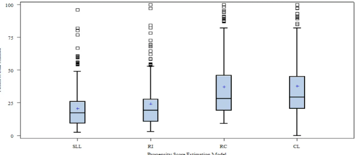
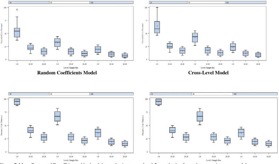
model ... 100 Figure 6: Mean percent of data trimmed by propensity score estimation model ... 102 Figure 7: Mean Percent of Data Trimmed by level-1 sample size across level 2-
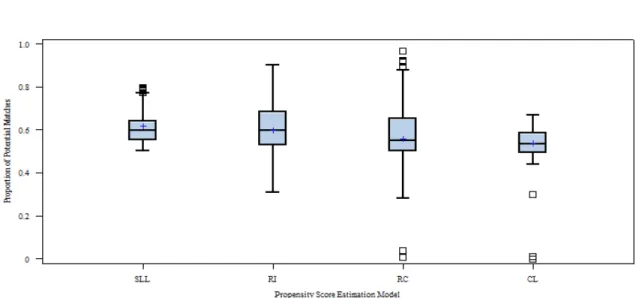
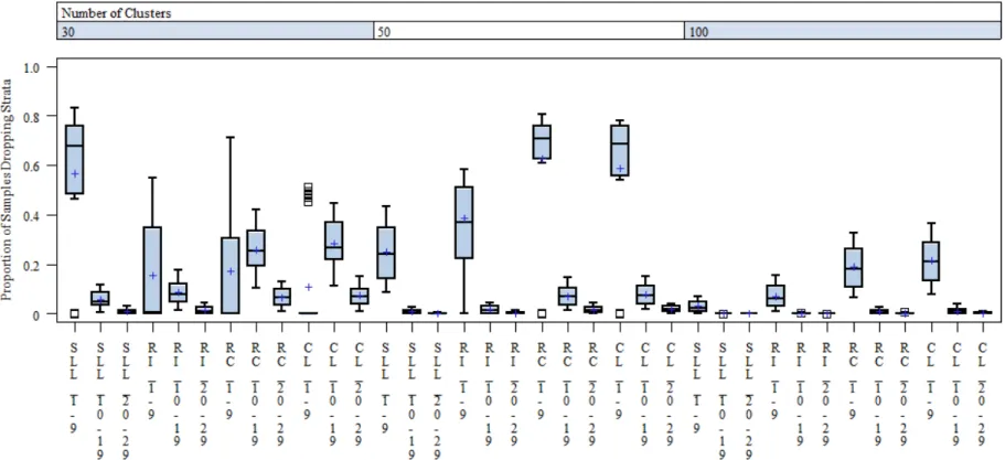
sample size for each propensity score model ... 103 Figure 8: Distributions of mean proportion of potential matches across PS models ... 106 Figure 9: Proportion of samples dropping strata by propensity score estimation model ... 107 Figure 10: Proportion of Samples Dropping Strata by the Sample Size Interaction
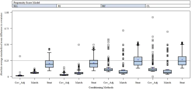
across the Four Propensity Score Models ... 109 Figure 11: Absolute average standardized mean difference in covariates by
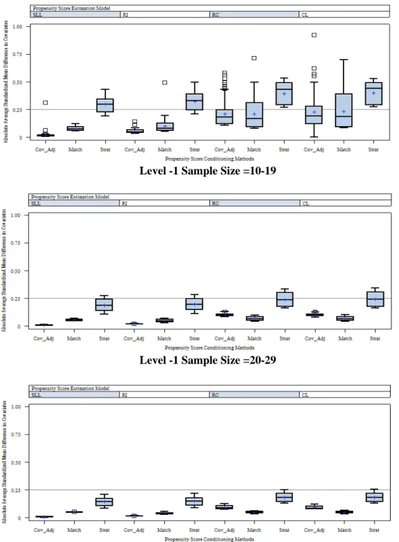
conditioning method across the four PS models ... 111 Figure 12: Distributions of the absolute average standardized mean difference in
covariates by conditioning method across the four PS models for each
level-1 sample size level ... 113 Figure 13: Absolute average standardized mean difference in covariates by
conditioning method across the four PS models for each level-2 sample size
level ... 114 Figure 14: Mean number of unbalanced covariates by conditioning method across the
four PS models ... 115 Figure 15: Distributions in mean number of unbalanced covariates by level-1 sample
vii
Figure 16: Distributions in mean number of unbalanced covariates by level-1 sample
size across conditioning methods by propensity score estimation model ... 117 Figure 17: Distributions of mean number of unbalanced covariates by conditioning
method across the four PS models for each level-2 sample size level ... 119 Figure 18: Proportion of samples balanced by conditioning method across PS
models ... 120 Figure 19: Proportion of samples balanced by conditioning method and level-1
sample size interaction across the level-2 sample size ... 121 Figure 20: Distributions of estimated bias in point estimates by conditioning
methods across PS models ... 123 Figure 21: Distributions of the average bias in point estimates by conditioning
method across the four PS models for each level-1 sample size level ... 125 Figure 22: Distributions of the RMSE for each conditioning method across the PS
estimation models ... 126 Figure 23: Root mean squared error for the level 1 sample size across the number of
clusters ... 127 Figure 24: Distributions of 95% confidence interval coverage rates for each
conditioning method across the four PS estimation models. ... 128 Figure 25: Distributions of 95% confidence interval coverage rates by level-1
sample size across the number of clusters ... 129 Figure 26: Distributions of 95% confidence interval coverage rates by PS estimation
models and conditioning methods across the number of clusters ... 131 Figure 27: Distributions of confidence interval width by conditioning methods across
PS estimation models. ... 132 Figure 28: Distributions of the confidence interval width by propensity score
estimation model and level-1 sample size interaction across the level-2
viii ABSTRACT
Propensity score analysis has been used to minimize the selection bias in
observational studies to identify causal relationships. A propensity score is an estimate of an individual’s probability of being placed in a treatment group given a set of covariates. Propensity score analysis aims to use the estimate to create balanced groups, akin to a randomized
experiment. This study used Monte Carlo methods to examine the appropriateness of using propensity score methods to achieve balance between groups on observed covariates and reproduce treatment effect estimates in multilevel studies. Specifically, this study examined the extent to which four different propensity score estimation models and three different propensity score conditioning methods produced balanced samples and reproduced the treatment effects with clustered data. One single-level logistic model and three multilevel models were investigated. Conditioning methods included: (a) covariance adjustment, (b) matching, and (c) stratification. Design factors investigated included: (a) level-1sample size, (b) level-2 sample size, (c) level-1 covariate relationship to treatment, (d) level-2 covariate relationship to treatment, (e) level-1 covariate relationship to outcome, (f) level-2 covariate relationship to outcome, and (g) population effect size. The results of this study suggest the degree to which propensity score analyses are able to create balanced groups and reproduce treatment effect estimates with clustered data is largely dependent upon the propensity score estimation model and conditioning method selected. Overall, the single-level logistic and random intercepts models fared slightly better than the more complex multilevel models while covariance adjustment and matching methods tended to be more stable in terms of balancing groups than stratification. Additionally,
ix
the results indicate propensity score analysis should not be conducted with small samples. Finally, this study did not identify an estimation model or conditioning method that was
1
CHAPTER ONE: INTRODUCTION
Causal Inference
Identifying causal relationships in social settings has been and continues to be a
challenge. Educational researchers often seek to identify causal relationships between programs, interventions, and/or treatments (herein "treatments") on various student outcomes, such as academic achievement (Austin, 2011; Chatterji, 2008; Slavin, 2002, 2008). Experiments investigate treatment effects of manipulable causes using statistical models to draw causal inferences. Manipulable causes are ones that can be deliberately altered or manipulated by the researcher, for example, participation in a program, method of teaching, or dosage amount. In contrast, non-manipulable agents such as gender cannot be deliberately altered and therefore, are not causes in experiments (Shadish, 2010; Shadish, Cook, & Campbell, 2002). Consequently, identifying causal relationships among non-manipulable variables becomes challenging (Shadish et al., 2002).
Causal relationships exist between two variables when the following hold true: (a) the cause precedes the effect, (b) the cause is related to the effect, and (c) no plausible alternative explanations for the effect exist other than the cause (Shadish et al., 2002). Treatment effects are estimated by a counterfactual model, or simply, the difference between what did happen after an individual received a treatment versus what would have happened if the same individual did not receive the treatment (Campbell & Stanley, 1963; Holland, 1986; Rubin, 2010; Shadish et al., 2002). Theoretically, causal effects can be precisely estimated if a unit was assigned to the treatment condition and the control condition at the same time in the same context. This would
2
allow outcome values for each unit under both of the conditions to be observed (Rubin, 1974, 1978).
In most field based settings, units can be assigned to one condition; therefore, only one outcome is observed —the outcome of the condition to which the individual was assigned. The unobserved or missing outcome is considered the counterfactual. For example, to investigate the effectiveness of a new reading program, an individual cannot be assigned to the new reading program and the old reading program simultaneously. The impossibility of observing both treatment and control outcomes for each individual is often referred to as the "Fundamental Problem of Causal Inference" (Holland, 1986, p. 947; Rubin, 1978).
Randomized controlled trials (RCTs), or randomized experiments, are considered the "gold standard" for estimating treatment effects (Austin, 2011; Cook, 2006; Donaldson & Christie, 2004; Education Sciences Reform Act [ESRA], 2002; Scriven, 2008; United States Department of Education [USDOE], 2003, 2005). In a randomized experiment, individuals are randomly assigned to treatment conditions. Random assignment allows groups to be
probabilistically similar, supporting a counterfactual inference; therefore, any measured differences in the outcome may be attributed to treatment effect (Campbell & Stanley, 1963; Games, 1990; Holland, 1986; Shadish, et al., 2002).
The process of randomization guarantees the two groups, on average, will be balanced at the beginning of the experiment, except for treatment assignment, and thus able to yield estimates of the average treatment effect (ATE). Estimates are considered to be unbiased because the randomization process ensures no plausible alternative explanation exists. Accordingly, well executed RCTs are able to produce unbiased estimates of treatment effects and are, therefore, the preferred method when investigating causal relationships. However, random assignment is often unethical or impractical in social and behavioral research. For example, to investigate the effectiveness of private school education on student achievement, the researcher is generally
3
unable to randomly assign students to private (treatment) or public (control) schools. Consequently, non-randomized studies are often used to estimate treatment effects (Austin, 2011).
In contrast,experiments which do not employ random assignment techniques, yet aim to explore causation, provide “less compelling support for counterfactual inferences” (Shadish, et al, 2002, p. 14) because groups are not probabilistically similar. In addition, causal relationships from non-manipulable variables may also be identified. Rubin (1979, 2001, 2007, & 2008) uses the term "observational studies" to refer to all studies aiming to explore causal relationship that do not incorporate the randomization process. Both non-randomized-experiments and
observational studies (herein non-randomized studies) lack the desired properties for causal inference and subsequently the validity of inferences are subject to various threats. These threats introduce sources of alternative explanations of the treatment effects which are thus considered to be potentially biased and less precise (Campbell & Stanley, 1963; Shadish, 2000; Shadish, et. al., 2002).
There are two basic approaches to addressing the estimation of causal effects in non-randomized studies: alternative design features (e.g. regression discontinuity, interrupted time-series) and applied statistical methods (e.g. ordinary regression, covariance adjustment analysis, structural equation modeling, selection models, and matching methods) (Gall, Gall, & Borg, 2007; Shadish, 2000; Shadish, et al., 2002; Stuart, 2010). Throughout the 20th century,
methodologists have worked to develop, refine, and evaluate these approaches. One of the more recent developments, introduced by Rosenbaum and Rubin (1983) is propensity score adjustment, a statistical method which aims to achieve balance between groups on a set of observed
4
Propensity Scores
A propensity score (PS) is the “conditional probability of assignment to a particular group, given a vector of covariates” (Rosenbaum & Rubin, 1983 p. 42). The purpose of the PS is to improve the quality of estimates from non-randomized experiments by attempting to mimic the balance between groups that occurs through the randomization process (Rosenbaum & Rubin, 1984; Shadish & Steiner, 2010; Stuart, 2010). The PS predicts an individual's probability for being assigned to the treatment group, thus ranges from 0 to 1. The closer the individual’s PS is to 1, the stronger the prediction for being in the treatment group; conversely, the closer the score is to 0, the stronger the prediction for being in the comparison group. When units from the treatment and control group have the same propensity score, it is assumed that the probability of being assigned to the treatment group is the same for each of these individual units, conditional upon the observed covariates. When there is no overlap in PSs between the groups, it is believed that the unobserved covariate(s) are accounting for the difference in groups (Stuart, 2010).
In randomized experiments, when treatment and control group samples have the same number of participants, the probability of being placed in treatment or control is equal (each participant’s PS = .50), and the two groups are considered to be comparable with differences being attributable to chance (Shadish & Steiner, 2010; Steiner & Cook, 2013). When
randomization is not possible, the probability of being placed in treatment or control is unknown but can be estimated. Equation 1 represents Rosenbaum and Rubin's (1983) formulation to represent an individual, i's probability of receiving the treatment, P (Zi=1), given a set of
observed covariates, X. The resulting probability, e(X), is the estimated PS:
( )
(
1|
)
i i i i
e X
=
P Z
=
X
(1)Estimating treatment effects using PSs is a multistep decision-based process that commonly includes the following procedures: (a) selecting the appropriate covariates related to both assignment and treatment to include in the model, (b) estimating the PSs, (c) conditioning on
5
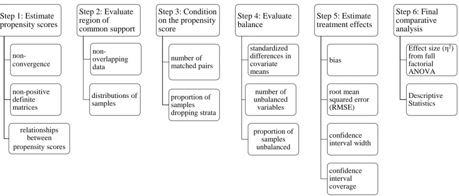
the PS, (d) assessing the accuracy of the PS estimation model, (e) adjusting the model if necessary, and finally, (f) estimating treatment effects (Rosenbaum & Rubin, 1983; Shadish & Steiner, 2010; Stuart, 2010) (see Figure 1).
Figure 1. Propensity score methodology framework.
Note: Figure is derived from Thoemmes, 2009, p. 150
Since Rosenbaum and Rubin’s seminal work in 1983, the study and application of PS has grown in popularity. Researchers have investigated the performance of PS techniques using Monte Carlo simulation studies (e.g. Austin, 2009; Gu & Rosenbaum, 1993) as well as existing databases (e.g. Michaelopoulos, Bloom, & Hill, 2004; Stuart & Green, 2008). Additionally, PSs have been applied to non-randomized studies across various fields including medicine (e.g. Murphy, Law, Whooley, Alexandrou, Chu, & Wong, 2003), business (e.g., Dehejia & Wahba, 1999), and social sciences (e.g. Hong & Yu, 2008).
Problem Statement
While RCTs may yield unbiased estimates of treatment effects, they are often difficult to implement in educational settings. Therefore, causal relationships in educational research are likely to be drawn from non-randomized studies which lack the desired properties to support counterfactual inferences and are highly vulnerable to threats to validity (Shadish et al., 2002).
Identify covariates to
include in the model
Estimate propensity
scores
Condition on the
propensity scores
Assess the PS model
and check balance
Possible revision and
reassessment of PS
model
Estimate treatment
effects
6
Because PSs aim to mimic certain characteristics of random assignment, their application is rapidly increasing. Historically, PS analysis has been used extensively in the medical field; however, recently it has begun to receive attention in other fields (Hahs-Vaugh & Onwuegbuzie, 2006; Pruzek, 2011; Thoemmes & Kim, 2011). Weitzen and colleagues (2004) investigated the PS estimation models considered by medical researchers, limiting their analysis to studies published during 2001 only. A total of 47 studies were ultimately included in their analysis. Similarly, Austin (2008a) also reviewed 47 studies published within the medical literature during 1996-2003. Austin (2008a) limited his analysis to applications employing only one conditioning method, matching. Reviews of PS applications in the social sciences have reported comparable numbers; however, these reviews did not impose strict criteria for inclusion and included a wider range of years across multiple disciplines. For example, Hahs-Vaugh & Onwuegbuzie (2006) searched the Education Resources Information Center (ERIC) database for educational studies applying PS techniques and identified a total of 25 applications of PS in education. Similarly, Thoemmes and Kim (2011) searched three large databases (ERIC, PsycINFO, and Web of Science), for PS applications in social science fields. Their search generated 111 studies
published from 1991-2008, of which, 86 met their inclusion criteria, and 34 were from education. The gradual adoption of PSs in the social sciences may be associated with the fact that there still remains a plethora of research situations for which there is a paucity of empirical evidence justifying the appropriateness of PSs (Shadish & Steiner, 2010). For example,
investigations of the behavior and application of PSs with nested data has received relatively little attention. Much of the research on PSs assumes observations to be independent (Arpino & Mealli, 2011; Hahs-Vaughn & Onwuegbuzie, 2006; Lingle, 2009); however, many systems, especially those in education, include a hierarchical structure where individuals are nested in multiple levels (e.g., students nested within classrooms; classrooms nested within schools; schools nested within districts) a violation of the independence assumption.
7
Hierarchical linear modeling (HLM), also referred to as multilevel modeling (MLM), is often employed when analyzing data with a nested or hierarchical structure (Raudenbush & Bryk, 2002). Estimating treatment effects within a nested context is complex because outcomes often depend upon contextual factors of the various levels. Additional challenges for drawing causal inferences within a MLM framework include implications associated with different hierarchical designs (Hong & Raudenbush, 2003). Currently, there is little guidance provided on how to incorporate statistical methods, such as PSs to draw causal inferences with nested structures (Thoemmes & West, 2011).
Recently, PS methods have been applied to studies conducted in multilevel settings (e.g., Hong & Raudenbush, 2005; Hong & Yu, 2008; Kim & Seltzer, 2007). Additionally, few studies have also recently begun to evaluate the performance of different PS methods with hierarchical data (Arpino & Mealli, 2011; Lingle, 2009; Rodriguez de Gil et al., 2012; Thoemmes, 2009; Thoemmes & West, 2011). While these studies have contributed to the body of knowledge, the literature on PSs with MLM remains sparse. Given the steady increase of PSs, coupled with the desire to investigate causal relationships in educational settings, further examination of the performance of PSs with MLM is warranted and timely.
Study Purpose
The purpose of this study was to further examine the appropriateness of using PS methods to achieve balance between groups on observed covariates and to yield unbiased treatment effect estimates in multilevel studies. Specifically, this study examined the extent to which different PS approaches (PS estimation models and PS conditioning techniques) and sample characteristics (sample size, covariate relationship to treatment and outcome, and population effect size) achieved balance and reproduced the population treatment effect.
PSs were estimated using four different logit models (a) single level model, (b) fixed slopes with random intercepts ignoring cluster-level predictors (random intercepts), (c) random
8
slopes and intercepts ignoring the cluster-level predictors (random coefficients) and, (d) random slopes and intercepts with cluster-level predictors added (cross-level). For each of the four PS estimation models, three different PS conditioning strategies were also investigated and included: (a) matching, (b) stratification, and (c) covariance adjustment. PS methods (estimation models and conditioning strategies) fully crossed with the sample characteristics were examined to evaluate the quality of balance achieved as well as the accuracy and precision of treatment effect estimates produced.
Research Questions
1. To what extent do balance estimates vary across PS methods (PS estimation models and PS conditioning strategies)?
2. To what extent do data factors (sample size, covariate relationship to treatment and outcome, and population effect size) affect the balance achieved by the PS methods (PS estimation models and PS conditioning strategies)?
3. To what extent do treatment effect estimates vary across PS methods (PS estimation models and PS conditioning strategies)?
4. To what extent do data factors (sample size, covariate relationship to treatment and outcome, and population effect size) affect the treatment effects estimated by the PS methods (PS estimation models and PS conditioning strategies)?
5. What is the direction and strength of the relationship between balance and both the accuracy and precision of treatment effect estimates?
Overview of the Study
This study incorporated Monte Carlo simulation methods to examine the performance of PS methods with MLM. Simulation methods allow for the control and manipulation of specific design and data factors to investigate the behavior of statistical methods (Guo & Fraser, 2010). This current study included nine design factors (see Table 1) related to either PS technique or
9
sample characteristics. These factors are (a) PS estimation models (single level, random intercepts, random coefficients, and cross-level); (b) PS conditioning strategies(matching,
stratification, and covariance adjustment); (c) number of clusters (small [n=30], moderate [n=50], and large [n=100]); (d) within-cluster sample size (small [n =01-09], moderate [n =10-19], and large [n =20-29]); (e) relationship between level-1 covariates and treatment assignment (small [βxz=.10], and moderate[βxz =.20 ]); (f) relationship between level-1 covariates and outcome (small [βxy =.10], and moderate [βxy=.20 ]); (g) relationship between level-2 covariates and treatment assignment (small [γwz =.20 ], and moderate [γwz =.40]); (h) relationship between level-2 covariates and outcome (small [γwy =.20 ], and moderate [γwy =.40]); and (i) population effect size (δ = small [0.2] and moderate [0.5]). All levels of all the factors were fully crossed with one another for a total of 288 data conditions (see Table 1). For each of the 288 data conditions, twelve different combinations of propensity score methods were conducted yielding a total of 3,456 conditions. For 254 out of 288 data conditions, 1000 datasets were simulated using SAS IML (SAS Institute Inc., 2008). The remaining 36 conditions, where the number of clusters was 100 and the number of level 1 units within these 100 clusters was large (20-29), 500 datasets were simulated using SAS IML (SAS Institute Inc., 2008).
Two specific aspects of PS methodology within a MLM framework were of interest in this study: the quality of the balance achieved and the accuracy and precision of the treatment effect estimates. The standardized differences for the estimated PSs and the observed covariates after conditioning were used to estimate balance. Outcome measures associated with effective treatment effect estimates included bias, standard error, 95% confidence interval coverage and width.
This study incorporates multiple analytical steps. First, PSs were estimated for each of the four models. Next, the PS estimates and samples were evaluated and trimmed to include only the common support areas. Then, each of the four PS model's trimmed samples were conditioned
10
Table 1
Design Features
Sample Characteristics PS Methods
PS estimation models Single level Random intercepts Random- coefficients Cross-level Sample size Covariate relationship to treatment Covariate relationship to outcome Population
effect size PS conditioning strategies* Number
of clusters
Sample size within
cluster
Level 2 Level 1 Level 2 Level 1
M S C M S C M S C M S C 30 01-09 10-19 20-29 γ0S=.20 γ0S=.40 β=.10 β=.20 γγ0S0S=.20 =.40 β=.10 β=.20 δ=.2 δ=.5 50 01-09 10-19 20-29 γ0S=.20 γ0S=.40 β=.10 β=.20 γγ0S0S=.20 =.40 β=.10 β=.20 δ=.2 δ=.5 100 01-09 10-19 20-29 γ0S=.20 γ0S=.40 β=.10 β=.20 γγ0S0S=.20 =.40 β=.10 β=.20 δ=.2 δ=.5 M= Matching S= Stratification C= Covariance Adjustment
11
three different times. Lastly, treatment effects were estimated using MLM, and balance on the conditioned samples was assessed. General Linear Models (GLM) procedures were conducted to address the research questions and draw inferences about the variability in balance and treatment effect estimates across PS methods and sample characteristics.
Delimitations
In addition to the manipulated factors, several design factors were held constant throughout this study. Data simulated included 27 continuous and 3 dichotomous level 1 covariates (X), 9 continuous and 1 dichotomous level 2 covariates (W), 1 binary assignment variable (Z) and 1 continuous outcome variable (Y). Data were generated so that the correlation between covariates within each level is approximately 0.2. Specific details regarding the three conditioning methods are presented in Table 2.
Table 2
Conditioning Methods
1. Matching - 1:1 Nearest neighbor caliper matching without replacement 2. Stratification- Five strata distributed evenly
3. Covariance Adjustment-including the estimated PS as varying level-1 covariate
Significance of the Study
Since the early 80's researchers have studied PS methods as well as multilevel models with respect to their ability to estimate effectiveness, individually. Many social and behavioral studies employ non-randomized studies in hierarchical settings to estimate treatment effects. Given that non-randomized studies lack the desirable properties of RCTs, it is imperative for methodologists to examine and improve methods used to identify causal relationships. The PS is a fairly recent statistical approach, and examinations of this method within MLM have received little attention. By examining the performance of PS in MLM, this study aimed to contribute to an important gap in the ongoing dialogue on causal inference in social and behavioral field settings.
12
Although recently researchers have begun to investigate the behavior of PSs with MLM through simulation studies, these studies have not considered conditions often found in applied educational settings. For example, previous studies have included relatively few level 1 predictors (e.g. less than 10) to balance groups (e.g. Arpino & Mealli, 2011; Lingle, 2009; Thoemmes & West 2011). In their review of PS applications in social science fields, Thoemmes and Kim (2011) reported an average of 31.3 covariates used in 79 studies. Inferences drawn based on investigations using ten covariates should be considered tentative when generalizing results to applications using more than ten.
The simulated samples in this study aimed to represent current applications of PS analyses in social science research and common attributes of educational data, specifically, focusing on research situations where units nested in clusters are assigned to treatment group with conditioning occurring across clusters. Several aspects distinguish the current study from
previous ones, particularly in sample complexity and PS methods investigated. Specifically the following characteristics induce a degree of complexity to the samples and have not previously been investigated within this context: (a) larger number of level-1 and level-2 predictors, (b) correlations among the predictors, and (c) dichotomous covariates. In addition, this study investigated a broad range of PS methods. For example, three different PS conditioning
techniques were examined in order to introduce and extend additional PS methods to a multilevel framework. Currently, little empirical evidence exists on which PS conditioning method work best under certain situations. Only a few studies compare the conditioning techniques using single level, non-nested data. No previous investigation of PS methods comparing three different conditioning techniques using MLM could be located. Lastly, the majority of methodological studies of PSs focus on the degree to which the PSs are able to remove bias in treatment effects; balance estimates are often a secondary outcome if and when included. Consequently, balance estimates are not consistently reported in applied studies incorporating PS methods (Thoemmes,
13
& Kim, 2011). Balance indicates the PSs' ability to create comparable groups that would mimic a random sampling design, an important, albeit overlooked purpose of PS models.
The findings from this study build upon the current literature and offer multiple avenues for future research. While this study's significant contributions are primarily methodological, current trends in social and behavioral research suggest the timely nature and opportunity for this study to provide applied researchers across disciplines additional information on the nature of causal inference with non-randomized nested data.
Limitations
Although this study contributes to the methodological literature on causal inference of non-randomized studies, specifically the use of propensity scores in multilevel contexts it is not without limitations. There are numerous combinations and permutations of potential design factors that may be considered. Data in this study was based on the specific aforementioned conditions and delimitations. While simulation studies are intended to provide evidence and rationale for empirical application, findings from this study can only be generalized to studies with similar conditions.
Definition of Terms
Assignment- binary variable that determines whether an individual or cluster receives
treatment or control.
Balance- met when the distribution of observed covariates is equal between treatment and
control groups.
Bias- the difference between a known parameter estimate and the estimated parameter
estimate
Common Support- the region of overlap in estimated PSs across treatment groups
Conditioning Strategies- methods employed to apply the propensity scores to balance the
14
Confidence Interval Coverage- the proportion of 95% confidence intervals that includes
the estimated parameter.
Confidence Interval Width- the difference between the upper and lower limits of the 95%
confidence intervals for the estimated parameter. This statistic will be aggregated across replications within each condition and represent the Average confidence interval width.
Confounding variable- a variable that is related to both treatment assignment and
outcome.
Control- the group not receiving or exposed to a specific condition under investigation of
its effectiveness. This group is often known as the referent group.
Counterfactual- the missing value that is estimated used by taking the differences in
observed outcomes in causal analysis.
Effectiveness -The change in a dependent variable that is attributed to a specific cause or
treatment.
Experiment- studies that investigate treatment effects of manipulable causes on specific
outcomes to provide evidence for causality.
Hierarchical Linear Modeling (HLM) - commonly referred to as multilevel modeling,
HLM is an analytic technique that is useful to examine data that are nested within one another such as students in classrooms, or teachers in schools.
Manipulable causes- Causes deliberately altered by the researcher when investigating the
effectiveness of treatments.
Non-manipulable variables- variables that cannot be controlled by the researcher and are
often included in as predictor or control variables.
Observational studies- studies that investigate causal relationships between
non-manipulable causes such as demographic variables and outcomes.
Percent non-overlapping data (PND) - the percentage of data for which the estimated PS
15
Propensity score- the “conditional probability of assignment to a particular group, given
a vector of covariates” (Rosenbaum & Rubin, 1983 p. 42)
Randomization- the process of using a random mechanism to assign subjects to treatment
conditions. This process ensures that groups are balanced on all observed and unobserved covariates and any differences are random.
Root Mean Squared Error- the square root of the average sums of squares of the errors.
Treatment- the group receiving or exposed to a specific condition under investigation of
16
CHAPTER TWO: LITERATURE REVIEW
This study investigated the behavior and performance of PS methods in multilevel settings. Accordingly, the review focuses on causal inferences using PS methods, and their appropriateness in multilevel studies. To provide a foundation the literature on causal inference, the theoretical framework for this study, is presented first. Included is a description of two distinct perspectives on the nature of causality. What follows is a discussion about the logic and use of PSs. Included here is a synthesis of current recommendations for applying PS methods within a single level context and a review of several empirical studies. Next, an overview to the theory and logic behind MLM is introduced. Lastly, research on PS in MLM will be discussed, empirical gaps will be identified, and a rationale for the proposed study will be offered.
Theoretical Framework
Originating as early as the 16th and 17th centuries, the concepts of causation and experimentation have influenced the development of Western Science in philosophy. Two distinct perspectives regarding the nature of causality and research are discussed within the literature: Rubin's Causal Model (RCM) and Campbell's validity framework. These two perspectives correspond to the two approaches to the estimation of causal effects in
non-randomized studies (applied statistical methods and alternative research features), respectively. RCM presents a framework for defining causal relationships and estimating treatment effects based on the counterfactual, sometimes referred to as potential outcomes (Holland, 1986). In contrast, Campbell's validity framework focuses on the inferences made from experiments and the potential threats to the validity of these inferences caused by various design related factors. Although often presented in isolation and operated independently rather than mutually (Shadish, 2010), these two perspectives are quite complimentary and share many common underlying
17
features (Rubin, 2010). RCM provides the foundation guiding the logic behind PSA while Campbell's commitment to improving causal inferences in non-randomized studies parallels the impetus of this study. Their unique perspectives provide a robust description of the theory of causality; thus, jointly serve as the theoretical framework for this study.
Rubin's Causal Model
RCM focuses on the precise mathematical and statistical properties related to causal inference, specifically the concept of potential outcomes (Rubin, 2010; West & Thoemmes, 2010). In RCM, treatment effects are determined by comparing the potential outcomes that would have been observed for an individual under different conditions. These outcomes are considered "potential" as each individual cannot be observed under various conditions simultaneously. In the simplest application of this model, there are two possible conditions (e.g. treatment and control) and each individual, i, has a potential outcome for each condition: Yi (0) for control and Yi (1) for
treatment. For each individual, the treatment effect, τ1, is defined as the difference between the
two outcomes:
τ1 = Yi (1) - Yi (0) (2)
Given this definition, it becomes impossible to observe both outcomes for the same individual. For each individual in the experiment, one of the two outcome variables will be observed, while the other one will be missing. Subsequently, it is impossible to find the
difference between the two outcomes for an individual, and the treatment effect for an individual can never be observed —the "Fundamental Problem of Causal Inference" (Holland, 1986, p. 947; Rubin, 1978).
RCM combats the fundamental problem using a statistical solution to estimate the ATE based on the expected value of the difference in outcomes, or a counterfactual model. Consider an experiment with two treatment levels, t (treatment) and c (control), where Z=1 when treatment is administered to an individual and Z=0 when the individual receives the control. Let Y
18
condition, and therefore only one outcome is observed; the outcome for the condition the individual was assigned. The unobserved outcome, or missing outcome, is considered the counterfactual. Equation 3 represents the observed outcome, Yi for an individual:
Yi = Zi Yi (1) + (1- Zi) Yi (0) (3)
In the counterfactual model, each individual will have one observed outcome Y,
dependent upon Z, and the counterfactual will be missing. Observed outcomes for each condition can be averaged, as these averages from the sample also correspond to the population average. The ATE of the population, U can be estimated from sample, u outcomes. The two distributions of observed outcomes Yz1 and Yz0 are formed by separate individuals and these distributions
represent hypothetical distributions of the population, had all individuals received treatment and control, respectively (Lunceford & Davidian, 2004). Consequently, the differences between the aggregated outcomes represent the ATE.
This solution to the fundamental problem allows causal inferences to be drawn using outcome measures observed from different individuals (Holland, 1986). In some situations, it is not the ATE that is of interest but rather the average treatment effect on the treated (ATT). For example, if students were able to elect to participate in an intensive dropout prevention program, the real interest here may not be the average effect, but rather the program's effect on those who participated. This is theoretically understood as the difference in outcomes with and without treatment for only those who were treated (Caliendo & Kopening, 2008; Holland, 1986; Rubin, 1973a, 1973b). Since outcomes for all treatment conditions cannot be observed for all units, RCM operates under several key assumptions discussed below (Rosenbaum & Rubin, 1983, 1984; Rubin, 2010).
Strongly ignorable treatment assignment assumption. Causal analysis and
counterfactual models rely heavily on the assumption of strongly ignorable treatment assignment, which when satisfied suggests alternative explanations have been accounted for and there is no hidden bias in treatment effects. This assumption refers to the mechanism or process used to
19
assign individuals to conditions and requires the assignment to condition be independent and not associated with the outcome or other factors. When satisfied, causal inferences can be drawn for population U using the average observed outcomes for all u in U exposed to t and c only
(Holland, 1986).
When u units are randomly assigned to conditions it is assumed that the cause of assignment mechanism Z, is statistically independent from the outcomes Yz1 and Yz0. This
assumption is considered to be satisfied through the randomization process; however, when randomization is not employed satisfying this assumption becomes complex as differences in observed outcomes may be attributed to alternative variables related to the assignment mechanism. Accordingly, well executed RCTs are able to produce unbiased estimates of
treatment effects and are, therefore, the preferred method when investigating causal relationships. The strongly ignorable treatment assignment assumption becomes a key factor regarding the quality of estimates in non-randomized studies. Ignorability of treatment assignment can be assumed if all the covariates that affect the treatment assignment have been accounted for, so that there are no unobserved covariates that may influence the estimates. If ignorability holds, one can obtain unbiased treatment effect estimates.
Stable unit treatment value assumption. Since outcomes for all treatment conditions cannot be observed for all units the outcomes from different units are compared. Therefore, experiments operate under the stable unit treatment value assumption (SUTVA), a strong
independence assumption. More formally, SUTVA is defined as an "a priori assumption that the value of Y for unit u when exposed to treatment t will be the same no matter what mechanism is used to assign treatment t to unit u and no matter what treatments the other units receive" (Rubin, 1986, p. 961). Simply, SUTVA assumes the outcomes from two individuals, irrespective of treatment assignment, are independent from one another. When operating under SUTVA, statistical solutions can be applied to estimate the ATE over a population (Holland, 1986).
20
Campbell's Validity Framework
Non-randomized studies lack desired properties for causal inference and when causal inferences are incorrect or invalid, there are several potential reasons for this imprecision,
referred to as "threats to validity" (Shadish et. al., 2002). Campbell's work focused on identifying the potential threats which often materialize in field settings and subsequently designing methods to account for them (Maxwell, 2010; Rubin, 2010; Shadish, 2010; West, & Thoemmes, 2010). A central focus of Campbell’s framework was his distinction of the two inferences made though experimentation. The first one being whether the independent variable or manipulable cause can produce a significant effect (internal validity), and the second one being the identification of the different populations, settings, variables, and conditions to generalize the significant effect (external validity) (Campbell, 1957).
The term internal validity has been adopted in the social sciences and psychological literature with meanings that vary from Campbell’s original definition (Shadish et al., 2002). In this context, internal validity refers to the extent to which the approximate truth is captured in an inference (Shadish et al., 2002). Validity can be considered a “property of the inferences” made, rather than a property of the design or methodology, because one design may yield more or less valid inferences in various circumstances (Shadish et. al 2002, p. 34). Cook and Campbell (1979) refined the distinction between internal and external validity and created a taxonomy of four different validity types to classify the different threats: (a) statistical conclusion validity, (b) internal validity, (c) construct validity and (d) external validity.
Statistical conclusion validity refers to the validity of the inferences about the covariation between treatment and outcome and answers the question regarding the strength, magnitude, and reliability of the covariation between the presumed cause and effect. Internal validity includes the threats associated to the validity of the inferences about whether the observed covariation between the treatment and the outcomes reflect a causal relationship from the treatment to the
21
outcome. Internal validity helps researchers understand whether the relationship was indeed causal or whether the outcome would have occurred regardless of exposure to the treatment. Construct validity is defined as the validity of the inferences about the higher order constructs representing sampling particulars such as the observed persons, the settings, and the cause and effect operations (Shadish et al., 2002). Construct validity allows researchers to identify the general constructs involved in the persons, settings, treatments and observations used in the experiment. Threats to construct validity identify a mismatch between the operations of the various particulars by the study and the constructs used to describe those operations. Lastly, external validity refers to whether the causal relationship holds over variation in persons, settings, treatment variables and measurement variables, or in other words the interaction effects. External validity specifically answers questions regarding the generalizability of the causal relationship over variation on the various sampling particulars.
The identification of specific potential threats within each of the four validity types has provided researchers with various sources that may be the culprit for the potential imprecision of the estimates generated from non-randomized studies. This process of ruling out threats to validity has been described as a “falsificationist enterprise” (Shadish et al., 2002, p. 41) where the purpose is to "reduce the number of plausible rival hypotheses" (Campbell & Stanley, 1963 p. 36) which would increase the "degree of confirmation" (p. 36) in the inferences. Arguably,
Campbell's most significant contribution was his quest to identifying the threats and developing research features to include in the study design in order to logically rule out plausible
explanations when conducting field based research (Rubin, 2010; Shadish, 2010; Shadish et al., 2002;West & Thoemmes, 2010) and provide a greater amount of trust for the causal inference in non-randomized experiments. Campbell and Stanley (1963) introduced the term
22
Causal Inference in Non-randomized Studies
Various statistical methods and procedures have been applied to adjust the data from observational studies to estimate causal relationship. Traditional matching methods, such as simple mean matching, pair matching (Rubin, 1973a) and multivariate matching (Rubin, 1976, 1979) are statistical methods that aim to equate the groups. Matching methods can be used to estimate both causal effects as well as non-causal relationships (Stuart, 2010). Traditional matching of individuals on relevant variables is complex.
As the number of related variables used to match increases, the number of combinations for individual matches between groups also increases exponentially (Cochran, 1965). For
example, if there are 10 dichotomous covariates, there are 1,024 combinations to match on. Thus, historically these methods allow for matching to be done on a limited number of covariates. Additionally, with traditional matching methods there is a potential to lose a lot of data. For example, in a study with 671 individuals assigned to treatment and 523 assigned to control; only 23 pairs were able to be matched on six categorical variables (Stuart, 2010). When few
covariates are used to match, estimates of treatment effects may seem unbiased (Cochran, & Rubin, 1973). However, the likelihood that one or two variables can account for the total variance explained by the treatment assignment is slim, and differences in treatment effects may be attributed to systematic differences between groups on variables not included.
In 1983, Rosenbaum and Rubin introduced the PS, a major advancement in causal analysis, specifically due to its ability to balance groups using a set of covariates reduced to a single score virtually eliminating the challenges with traditional matching (Shadish & Steiner, 2010). The ability to include many variables increases the likelihood of satisfying the strong ignorability assumption. When the assumption of strongly ignorable treatment assignment holds PSs can yield unbiased treatment effects (Stuart, 2010; Shadish & Steiner, 2010).
23
The Logic of Propensity Scores
Rosenbaum and Rubin (1983) introduced the concept of using balancing scores to group treatment and control units in non-randomized studies. A balancing score is defined as the "function of observed covariates, such that the conditional distribution of these observed covariates is the same for treated and control units" (Rosenbaum & Rubin, 1983, p. 42). For example, balancing score, b(x), is a function of the observed covariates, x (Rosenbaum & Rubin, 1983). Individual units assigned to different conditions with the same, b(x), are assumed to be comparable, therefore using balancing scores may mimic the properties of a randomized
experiment, where groups are considered to be probabilistically similar. In other words, balance implies that the variables x, are statistically independent of treatment assignment; therefore cannot be a confounding influence and unbiased estimates of the treatment effect are possible, assuming no other confounders exist. Rosenbaum and Rubin (1983) introduced the PS, as a specific and coarse type of balancing score that collapses a set of covariates into a single score to balance the groups.
Rosenbaum and Rubin (1983) proved that if the PSs are balanced between the two groups, then all the covariates used to estimate the PS are also balanced on average in large samples. Therefore, when conditioning on the balanced PS estimates, the covariates are statistically independent of treatment assignment, thereby mimicking the expected properties of randomized experiments potentially producing unbiased treatment effect estimates. A key assumption of PSs and their capability for producing unbiased estimates is that x, the vector of covariates, contains all variables that may potentially bias the treatment effect estimate. More simply, PSs rely heavily on the strongly ignorable treatment assignment assumption (Rosenbaum & Rubin, 1983). The process of applying PS to estimate treatment effects requires multiple decision-based steps. These steps are described in detail below.
24
Covariate selection
The selection and inclusion of appropriate covariates is an integral component in PS. The quality of the estimated PS depends upon its ability to remove hidden bias which is a function of the covariates included in the model. PS relies heavily upon the assumption of ignorable
treatment assignment; therefore, in order to satisfy the ignorable assumption all variables related to treatment and outcome need to be included (Rubin & Thomas, 1996; Stuart, 2010). There is no statistical test for this assumption; its satisfaction is inferred through substantive knowledge of the possible confounding variables in the applied context (Shadish & Steiner, 2010; Stuart, 2010; Steiner, Cook, Shadish, & Clark, 2010). Therefore, even if a large number of covariates are included, there is no way to tell whether a confounding variable has been excluded, or overlooked. Bias from unobserved covariates is known as hidden bias (Guo & Fraser, 2010; Rosenbaum, 1987, 2002). The researcher is confronted with the responsibility of selecting the appropriate variables to satisfy the strongly ignorable treatment assumption. If important covariates related to treatment assignment are omitted, then there is potential for the PS to be biased, thus the resulting treatment effect estimates will also be biased (Rubin, 1997; Shadish & Steiner, 2010). The exclusion of potential confounding variables impacts the treatment effect estimates and consequently threatens the validity of the inferences (Rosenbaum & Rubin, 1983; Shadish & Steiner, 2010; Steiner, Cook, & Shadish, 2011; Stuart, 2010).
Estimation Methods
There are two basic methods for estimating propensity scores: binomial regression models and statistical learning algorithms (Shadish & Steiner, 2010). Binomial regression models, such as logistic regression models or probit models, belong to the large family of models known as generalized linear models and are currently the most common method of PS estimation (Shadish & Steiner, 2010). Generalized linear modeling (GLM) is a technique for modeling data with non-normally distributed response variables, such as binomial distributions (Agresti, 1996; McCullough & Nelder, 1989; Nelder &Wedderburn, 1972; Quinn & Keough, 2001).
25
GLM's, specifically logistic models, consist of three components. First is a random component, which is the response variable and its probability distribution, second is the systematic component which is represented by the predictors or covariates used to specify the model, and third is the link function which is used to connect the random and systematic
components (Agresti, 1996; Quinn & Keough, 2001). The most common link function for binary data and logistic regression is the logit link which transforms the predicted probabilities into logits or the natural log of the odds. Thus, in multiple logistic regression a set of k predictors for a binary response Y is modeled so that the logit of the probability, π, that Y=1 can be generalized using the following equation:
[ ]
0 1 1 logit log ... 1 x nxnπ
π
β
β
β
π
= = + + − (4)Here, β0 is the average PS for the sample or the average probability in logit units of receiving treatment across individuals assuming all the covariates are centered and normally distributed. The parameter β1 refers to the effect of X1 on the log odds that Y=1 controlling for
the other Xs (Agresti, 1996, Hosmer & Lemeshow, 2000). The logit link is considered favorable because the probabilities are modeled as a linear function of the covariates and the outcome, the natural log of the odds is a continuous, normally distributed variable (O'Connell & Rivet Amico, 2010). In the context of PS analysis, logistic regression models estimate the probability of being assigned to the treatment, conditional on the covariates specified.
With logistic regression models, least squares estimation for the model parameters are not optimal, because the variance of the binary outcome for each individual is not constant across all predictors, but rather depends on the probability for each predictor (Agresti, 1996). With the non-constant variance, maximum likelihood (ML) estimates can yield smaller standard errors than least squares estimates; therefore, ML estimation is used in logistic models (Agresti, 1996; O'Connell & Rivet Amico, 2010; Quinn & Keough, 2010).
26
Statistical learning algorithms also known as machine learning or ensemble methods refer to techniques such as classification or regression trees, boosting, bagging, or random forests (Shadish & Steiner, 2010). These methods try to iteratively minimize imbalance in covariates, while taking into account any nonlinear relationship between covariates and treatment assignment (McCaffrey, Ridgeway, & Morral, 2004). For example, a classification tree uses a recursive algorithm to estimate a function describing the relationship between a multivariate set of
independent variables and a single dependent variable, for example treatment assignment. Using one variable as its basis, the tree fitting algorithm splits the dataset into two regions. The chosen split is the one that minimizes the prediction error. Within a region defined by its splits, the estimated function is equal to the sample mean of the outcome variable for all observations that based on the value of their covariate are included within the region. The regions are each
subsequently partitioned and this process occurs iteratively until the number of allowable splits is reached (McCaffrey et al., 2004).
Since PSs are meant to create comparable groups, after PSs have been estimated, it is good practice to assess the two groups based on their estimated PSs. One method is to examine the distribution of the estimated PSs between the groups, known as the region of overlap or common support region (Shadish & Steiner, 2010; Stuart, 2010; Thoemmes & Kim, 2011). A broad region of common support allows for causal effect estimates to be based on the full range of PSs in the sample, whereas a small common support region restricts the effect estimates. Often individuals who have estimated PSs that fall outside the common support region are dropped from the analysis. These individuals are usually located in the tails of the distribution, with estimated PSs close to 1 and 0. If PSs yield insufficient overlap then it may be that the model to estimate the PSs needs to be adjusted.
Conditioning methods
Once PSs are estimated, the next step is to utilize, or condition on them to balance the treatment and control groups. There are four general conditioning techniques: matching,