Global, non-parametric, non-iterative optimization of
time-averaged quantities under small, time-varying forcing: An
application to a thermal convection field
Hideshi Ishida∗
Department of Mechanical Engineering,
Faculty of Science and Engineering, Setsunan University,
17-8 Ikeda-Nakamachi, Neyagawa, Osaka 572-8508, Japan
Shiho Ihara,† Chiharu Okema,‡ Shohei Yamada,§ and Genta Kawahara
Department of Mechanical Science and Bioengineering,
Graduate School of Engineering Science, Osaka University,
1-3 Machikaneyama-cho, Toyonaka, Osaka 560-8531, Japan
Abstract
This study demonstrates a global, non-parametric, non-iterative optimization of time-mean value
of a kind of index vibrated by time-varying forcing. It is based on the fact that the (steady) forced
vibration of non-autonomous ordinary differential equation systems is well approximated by an
analytical solution when the amplitude of forcing is sufficiently small and its base state without
forcing is linearly stable and steady. It is applied to optimize a time-averaged heat-transfer rate
on a two-dimensional thermal convection field in a square cavity with horizontal temperature
difference, and the globally optimal way of vibrational forcing, i.e. the globally optimal, spatial
distribution of vibrational heat and vorticity sources, is first obtained. The maximized vibrational
thermal convection corresponds well to the state of internal gravity wave resonance. In contrast,
the minimized thermal convection is weak, keeping the boundary layers on both sidewalls thick.
† Present address: All Nippon Airways Co., Ltd., Shiodome-City Center, 1-5-2 Higashi-Shimbashi,
Minato-ku, Tokyo 105-7140, Japan
‡ Present address: Daikin Industries, Ltd., Umeda Center Bldg., 2-4-12 Nakazaki-Nishi, Kita-ku, Osaka
530-8323, Japan
§ Present address: DENSO Corporation, 1-1 Showa-cho, Kariya, Aichi 448-8661, Japan
Nomenclature
a amplitude of time-dependent forcing v y-direction velocity component
b (complex) vibrational vector field v vector field of an autonomous system
ˆ
b (complex) vibrational form x a point on a phase space
d a vector to introduce a index ˆx base state, stable steady thermal
f (complex) external forcing term convection field
G third rank tensor, defined by Y admittance matrix
Gijk≡∂2vi/∂xj∂xk Greek symbols
ˆ
G a matrix, ˆGαβ ≡diY(0)ijG(xˆ)jαβ. α inner-product of a optimal
Gr the Grashof number vibrational form and a feasible
H a matrix,H(ω)≡Y∗(ω) ˆGY(ω) one
I (inner-product-type) indicator σ a positive constant
I time-mean value of I θ temperature
J Jacobian matrix of a vector fieldv ω angular frequency of vibration
M Jacobian matrix of a vector fieldb ζ vorticity
N division number Subscripts
N u (surface-averaged) Nusselt number a first-order correction
P r Prandtl number,ν/χ aa second-order correction
Ra Rayleigh number Superscripts
Sθ vibrational heat source * conjugate transpose
Sζ vibrational vorticity source opt optimized (maximized or
t time minimized) quantity
u x-direction velocity component
I. INTRODUCTION
vorticity [8] and velocity [9, 10], drag reductions [11, 12], heat transfer rates [13–17, 21–24], shear stresses [18–20] and so on. However, most of them are parametric optimization, useful in cases where the number of optimization variables is small. Like the field optimization [25–27], however, large or infinite number of the variables prevents us from utilizing the method.
That is the reason why non-parametric methods are applied to solve the types of op-timization. However, very little work is available for optimizing time-averaged quantities because of the difficulty of unsteady optimization [28–34]. Srinath and Mittal [28] and Fang and Li [33] applied a continuous adjoint method to obtain the optimal shape of airfoils for maximizing time-averaged lift coefficient or minimizing time-averaged drag coefficient, in conjunction with iterative methods, such as descent or conjugate gradient methods. Simi-larly, iterative algorithms were utilized to maximize time-averaged system energy efficiency [29], and to maximize time-averaged transmission rate [32], and so on.
The use of iterative methods is inevitable for the cases governed by nonlinear equations: the optimal solution cannot be obtained by a one-time numerical computation. Accordingly, the application of non-parametric and non-iterative optimizations of time-averaged quanti-ties are limited to special cases to which analytical approaches are useful [35, 36]. Nelson et al. [35] proposed the active control of low-frequency random sound in enclosures and, as an example, it is applied to one-dimensional enclosure to minimize time-averaged acoustic potential with the aid of an analytically obtained auto-correlation function. Chen and Muga [36] studied a time-dependent harmonic oscillator and found that the time-averaged energy realized by the optimal, time-dependent engineered scaling function is indeed minimum, reaching its lower bound obtained analytically. In general, however, even if such an optimal solution is obtained, we do not know whether or not the solution is globally optimal. We more or less confront these issues to optimize over a field for maximizing or minimizing a time-averaged quantity.
forcing on the same base field given by a non-vibrational condition. As long as the base field is linearly stable, steady state, the perturbation expansion is possible, and its second-order truncated expansion [38] provides us with the above-mentioned optimization method. Discretization of governing equations makes it possible for us to apply the method to many practical systems with damping mechanisms and holonomic constraints, and to obtain the globally optimal vibrational field without any parametric, iterative computations.
As an application of the field-optimization method, we are to address a vibrational ther-mal convection [39–46] with a horizontal temperature difference in a square cavity, and time-mean heat transfer rate, i.e. Nusselt’s number, is maximized and minimized. Recently, Pourgholam et al. [17] found that the time-averaged heat transfer rate on the heated top and bottom walls in a parallel flow channel reaches maximum by a periodically moving blade near the inlet port. Velazquez, Arias and Mendez [16] showed that the maximum time-averaged Nusselt number over the downstream portion of a backward facing step is 55% larger than the value of the steady state when velocity modulation is exerted in the inlet port at the resonant frequency. Such a heat transfer maximization induced by external vibrations is rather intensely examined in natural convections [40–46]. For instance, Kim, Kim and Choi [44] conducted a numerical study to investigate the boundary layer instability in a square cavity with side-wall temperature modulation, and clarified that the maximum time-averaged heat transfer rate is obtained for the oscillation in tune with the frequency of boundary layer instability. They are parametric optimizations with smaller numbers of optimization variables and, to our best knowledge, the spatial distribution of vibrational heat and vorticity sources to optimize the time-averaged Nusselt number is first obtained in this study. The maximization and minimization are simultaneously accomplished by solving an eigenvalue problem of a Hermitian matrix.
here.
II. METHODS AND DEFINITIONS
A. Approximation of forced oscillation on ODEs
Considering that a partial differential equation system with holonomic constraints is discretized to be an ordinary differential equation system (ODEs), it is meaningful for us to begin with the following system with forcing
dx
dt =v(x) +af(x, t), (1)
where x denotes a column vector of N components indicating a point on a phase space,
f forcing normalized by the amplitude a, and v vector field without forcing. We assume that it has a linearly stable, steady solution ˆxwhen a= 0, hereafter referred to as the base state, and that the amplitude a is sufficiently small. Then taking a to be a perturbation parameter, we are to solve the equation around the steady solution of the form
x=ˆx+axa+a2xaa+· · · . (2)
We can obtain the corrections such as xa and xaa analytically. The procedure is detailed in
Ref. [38]. In what follows, we are to restrict the vibrational forcing f into a single-frequency vibration of the form
f =eiωtb(x) +c.c., (3)
where ω denotes angular frequency of vibration, b a complex vibrational vector field, and
c.c. the complex conjugate terms. Then the steady responses of the first- and second-order corrections are given by
xa=eiωtY(ω)ˆb+c.c., (4a)
xaa =e2iωtY(2ω)(bˆTYT(ω)G(ˆx) + 2M(ˆx))Y(ω)ˆb/2
where ˆb ≡ b(ˆx), and Y ≡ (iωI −J(ˆx))−1, and the overline denotes complex conjugate
quantities [38]. A third rank tensor G is defined by Gijk ≡∂2vi/∂xj∂xk, and its associated
operation is also defined as xTGy
i ≡Gijkxjyk. I denotes the identity matrix, and J and
M denote the Jacobian matrices of vand b, respectively. As long as the (steady) base field
ˆ
x is linearly stable, i.e. all of the real parts of the eigenvalues of J(ˆx) are negative, the (impedance) matrix iωI −J(ˆx) is regular and, therefore, the correction terms are bounded for any real number ω.
The tensors J(xˆ), Y(ω) and G(ˆx) are intrinsic properties of a given vector field v and a base field xˆ without forcing. Y is referred to as an admittance matrix in Ref. [37], corresponding to a frequency response function. In contrast, the complex matrix M(ˆx) and vector bˆ have the information on the way of vibration, and bˆ is hereafter referred to as vibrational form. This is the optimization variable in this study.
When the expansion (2) is truncated at the first- or second-order, the perturbation ex-pansion becomes the first- or second-order approximation with respect to the vibration amplitudea[38]. Particularly, the second-order approximation has a correction term for the direct-current component caused nonlinearly by a vibrational forcing, making it possible to treat the change in time-mean values by vibration. By modifying two variables M(ˆx) and
ˆ
b, we obtain the response to an arbitrary small-amplitude time-varying forcing.
In order to apply these approximations, the amplitude a must be small enough, math-ematically infinitesimal. The applicability of the truncated forms will be examined in Sec. III A.
B. Optimization and formalism
On the first-order approximation, i.e. first-order truncated perturbation expansion, Ishida et al. [37] showed that the maximization of total amplitude, defined by |Yb|2, subject to the normalization condition of vibrational form ˆb, is reduced to an eigenvalue problem of a Hermitian matrix ˆH(≡Y∗Y), where superscripted asterisk0∗0 denotes conjugate transpose.
1. Inner-product type index and the optimization of its time-averaged quantity
The quantity is an inner-product-type index I, defined by
I ≡dTx, (5)
where d is a constant real vector. For its time-mean value ¯I¯we consider the problem
maximize (minimize) ¯I¯(ˆb, M(ˆx), ∂2bi/∂xj∂xk(ˆx),· · ·)
subject to
ˆ b
2 ≡
ˆ b
2
/σ = 1, (6)
M(xˆ) = 0,
where σ is a positive constant. As we shall see, the following formulation is unchanged on the condition that the L2-norm of bˆ is held fixed. The constant σ may be interpreted in
such a degree of freedom. The restriction of the vibrational way to the case of M(ˆx) = 0 is for simplification in this study.
On the second-order approximation, ¯I¯is a function ofbˆ(andM(ˆx)) only, and the problem is reduced to the following eigenvalue problem of a Hermitian matrix H:
Hbˆopt =λoptbˆopt, (7)
where
H(ω)≡Y∗(ω) ˆGY(ω),
ˆ
Gαβ ≡diY(0)ijG(ˆx)jαβ,
and the optimized value of ¯I¯can be expressed as
¯ ¯
Iopt =dTˆx+a2σλopt
ˆ
bopt
2
, (8)
whereλopt is the maximum or minimum eigenvalue of the problem (7), and ˆbopt is its
and corresponding vibrational forms are obtained at the same time without any parametric, iterative computations and that they are the globally, not locally, optimal solutions.
Some reasonable constraints of vibrational form can change the the definition (6) of the norm into the form
ˆ b
2 ≡ 1
σ ˆ
b∗Aˆb, (9)
where A is a positive definite Hermitian matrix. In this case, the optimization problem is reduced to the following generalized eigenvalue problem:
Hbˆopt =λoptAbˆopt, (10)
and the formulation provides again a non-parametric, non-iterative optimization procedure. For simplification, however, we shall not treat such a case of constraint in this study.
C. A sample vector field: a thermal convection
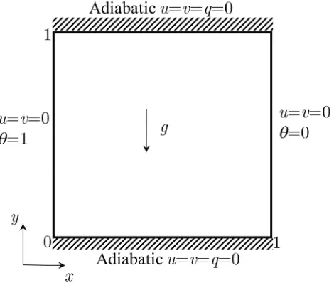
A base and a vector fields are needed to assess the applicability of the optimization scheme. The sample base field in this study is a two-dimensional, dimensionless thermal convection in a square cavity shown in Fig. 1. A constant temperature difference, not constant heat flux [37, 38], is given between the left- and right-hand side walls so that time-mean heat transfer rate can be changed by vibrational forcings. The top and bottom walls are insulated. The no-slip, zero velocity condition is set on the wall surfaces. The gravity works in the negative y direction.
A phase space is defined by use of vorticity ζ and temperature θ defined at inner lattice points within the cavity: when we define ζi and θi for a natural number i, as described in
Fig. 2, a sample coordinate xof a phase space can be defined as
x≡(ζ1, ζ2,· · · , ζL, θ1, θ2,· · · , θL).
In this study the division numbers n and m for horizontal and vertical directions, respec-tively, are equal, i.e. n =m(≡N).
be-haves like a holonomic constraint [37, 38]. In this study these equations are discretized by finite difference method, expressed by the vorticities and temperatures defined on the above-mentioned inner lattice points with the aid of the boundary conditions. Convection and diffusion terms are discretized by QUICK and central difference schemes, respectively. Consequently, we obtain a vector field v of x.
In this study, the Prandtl numberP r, the Rayleigh number Ra, and the Grashof number
Gr(≡Ra/P r) are fixed at 0.71, 105 and 1.4×10⁵, respectively, so that non-vibrational field
evolves to reach a stable steady state of a clockwise-rotation circulatory flow. It is the base state, denoted by ˆx, on which vibrational forcings are imposed.
The present introduction of vector and base fields, v and ˆx, allows us to apply the optimization theory explained in the previous section. In the theory, however, the way of vibrational forcing is restricted to the case that M(ˆx) = 0. Then the optimal vibrational form ˆbopt obtained corresponds to the optimal spatial distribution of the following complex
vibrational vorticity sourceSζ and heat sourceSθ, included in the vorticity and temperature
equations:
∂ζ
∂t +
∂(uζ)
∂x +
∂(vζ)
∂y =Gr
∂θ
∂x + ∆ζ+ae
iωtS
ζ(x, y) +c.c., (11a)
∂θ
∂t +
∂(uθ)
∂x +
∂(vθ)
∂y =
1
P r∆θ+ae
iωtS
θ(x, y) +c.c. (11b)
The optimization method makes it possible to have the spatial distribution without any parametric studies.
For a normalization condition, the positive constant σ in Eq. (6) must be σ = N2 so
that the sum of spatial integral of absolute value squared of the sources would be constant at unity as the division number N tends to infinity, that is
lim N→∞ ˆ b 2 = Z V
(c|Sζ| 2
+|Sθ| 2
)dV = 1, (12)
Other reasonable constraints can modify the definition of the norm. Providing it has the form of Eq. (9), including the above norm (12), we can instead solve the eigenvalue problem (10) and obtain a optimal solution depending on the norm. For instance, time-averaged quantity of spatially integrated enstrophy on the domain corresponds to the time-averaged energy input. Based on the first-order approximation, the constraint of fixing the input is of the form (9). Let us confirm herein that the main objective of this study is to present such a general framework of non-parametric, non-iterative optimization on ODEs (1).
III. RESULTS AND DISCUSSIONS
Given the vector field v and a vibrational form, we can confirm the applicability of the approximations and the optimization theory, introduced in the previous section. First of all, the second-order approximation is numerically validated by comparison with a direct computation without any approximations. Such a validation has already been made on a base state with a constant heat-flux on the left-hand side wall [37, 38]. In this section, it is validated for a base state with a constant temperature on the sidewall, based on the boundary condition of this study. Next, the thermal convections optimizing dimensionless heat transfer rate, Nusselt’s number, are presented and, finally, we confirm they are indeed optimal solutions by use of direct computations.
A. Numerical validation of approximated solutions
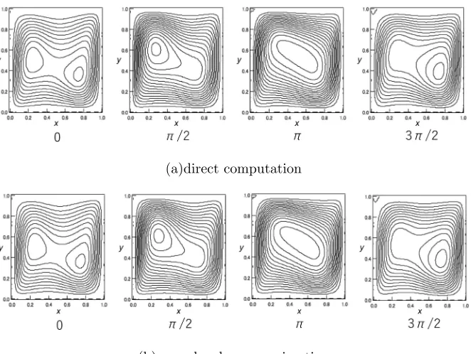
Figure 3 shows steady response of streamfunctions to a left-hand sidewall temperature variation, given byθ|x=0 = 1+asinωt, wherea= 0.2,ω=250, and division numberN = 100.
The flow fields obtained by the second-order approximation are in good agreement with those by the direct computation.
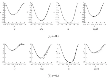
third-order approximation is better than the second-third-order one for some phases. In total, however, the second-order approximation well recovers the results of direct computations while the amplitude a is sufficiently small, i.e. a≤0.4.
Herein, please note that whether or not the amplitude a is small enough depends on the way of vibration, quantified by M(ˆx) and vibrational form ˆb. The larger the norm of these quantities, the smaller the amplitudea should be. For the case of the present vibration, the norm of bˆ is very large, evaluated to be the order of 103 (N3/2), diverging as N tends to
infinity. Moreover, it is well known that the base thermal convection field of this study has an intrinsic vibrational mode of internal gravity wave (IGW) [47–49], caused by density or temperature gradient in the direction of gravity acceleration. The natural frequency in a rectangular cavity has been obtained by Thorpe [48] for inviscid fluid, estimated at around
ω = 250 in the present square cavity. Therefore, the amplitude of forced oscillations can be relatively large at this frequency. Taking these issues into consideration, we can expect that the second-order approximation is applicable in many practical situations.
B. Optimization of time-mean Nusselt’s number
We can easily confirm that the (surface-averaged) Nusselt number N u on the left-hand side wall is a function of a phase (state) point x, introduced in Sec. II C, of the form
N u(x) = C+dTx with a constant C. Thus the optimization of time-mean value of N u,
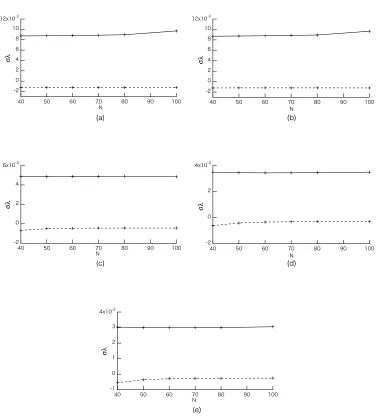
subject to the constraint (6) on the vibrational formbˆ, is reduced to the eigenvalue problem (7). The largest and smallest eigenvalues are shown in Fig. 5. The optimized Nusselt number N uopt is expressed by the optimal eigenvalue λopt (λmaxorλmin) as follows
N uopt =N u(ˆx) +a2σλopt
ˆ
bopt
2
,
and the optimal vibrational form ˆbopt is its corresponding eigenvector. If the optimal form
converges as N approaches infinity by an appropriate definition of its norm, and also if the optimal Nusselt number converges by the property of the Boussinesq equation system, the value σλopt also does. That is the reason why the vertical axis in the figure is taken to be
σλ.
properties of the Boussinesq equation system, independent of the division numberN. Figure 6 shows the distribution of optimal vibrational heat source to maximize N u at
ω = 240. We can confirm that its amplitude converges sufficiently at N = 60, and that its phase is also in the process of convergence. They are also regarded as the optimal properties of the Boussinesq equation system.
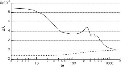
The dependency of the optimal eigenvalue on the angular frequencyω is shown in Fig. 7. The minimum eigenvalue is monotone increasing and approaches to zero withω. In contrast, the maximum value has three local maxima at ω = 240, 360 and 450, which includes the above-explained natural frequency of IGW.
The frequencies can be explained by the linear stability analysis of the steady solution ˆx. Figure 8 shows the result of eigenvalue analysis of J(ˆx). Among Hopf modes with complex eigenvalues, the imaginary parts of three eigenvalues that have relatively large real parts agree well with the three angular frequencies. Similar coincidence has been reported in our previous study [37] of the case of total amplitude maximization. At all events, the intrinsic vibrational modes of base state ˆx are reflected in the imaginary parts, and the maxima of Nusselt’s number can be caused by the nonlinear effects of the optimal large-amplitude forced oscillation imposed on the intrinsic modes.
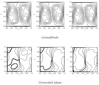
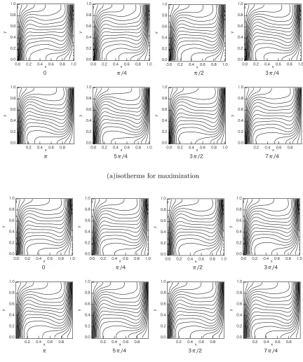
At the angular frequency of IGW (ω = 240), the optimal forced oscillation are shown in Fig. 9. The maximized thermal convection inclines isotherms to the right side at a phase while it does not incline isotherms to the left side, keeping on average the thermal boundary layer near sidewalls thin. Conversely, the minimized thermal convection is weak, keeping in total the boundary layer thick.
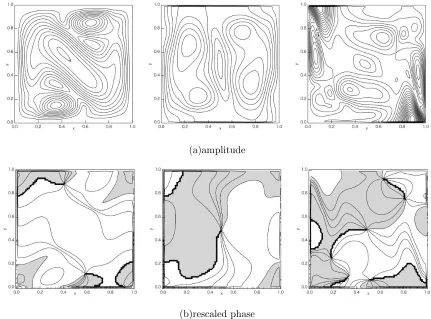
The vibrational form, i.e. vibrational heat and vorticity sources, to induce such thermal convections are shown in Fig. 10. As (the increment of) the amplitude of the vorticity source is tiny, the above-mentioned thermal convections are dominated by the buoyancy force associated with vibrational heat source. The source for maximization has two peaks on right and left halves, and they are antiphase as shown in the distribution of rescaled phase. They are similar to the distribution to resonate with IGW [37], which causes alternative inclinations of isotherms.
C. Application and validation of optimization method
The optimal vibrational form, i.e. optimal vibrational vorticity and heat sources, provides us with vast pieces of information to realize the optimal vibration as much as possible. For the present physical model, the vibrational heat source is realized by the Peltier device and, fortunately, the vorticity source can be negligible. Referring to the vibrational form bˆ(optmax)
for maximization (Fig. 10), we consider the following simple, feasible vibrational form bˆ0,
defined by
Sζ = 0, (13a)
Sθ =
1/(√2∆); 0.05≤x≤0.05 + ∆, 0.65≤y≤0.65 + ∆,
−1/(√2∆); 0.65≤x≤0.65 + ∆, 0.05≤y≤0.05 + ∆,
0; elsewhere,
(13b)
where ∆ = 0.3. As explained in the previous section, the vibrational heat source mimics the optimal one that has two antiphase peaks near upper-left and lower-right corners. The linearly independent, normalized vibrational forms, ˆb(optmax) and bˆ0, span a two-dimensional
vector space. In this section, we consider a normalized vibrational formbˆ(s) of a real variable
s (−1≤s≤1) to connect continuously between the two vectors on the space, defined by
ˆ
b(s) = s
s0
ˆ
b0+ (
α
|α| √
1−s2− s
s0
α)bˆ(optmax), (14)
where
α=bˆ(optmax)∗bˆ0 ≡(bˆ(optmax),bˆ0)
and
s0 =
q
1− |α|2.
Herein, the parameter s corresponds to the sine of the angle between the vectors bˆ and
ˆ
ˆ
b(0) = α
|α|bˆ (max)
opt ,
ˆ
b(s0) =bˆ0.
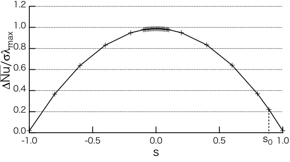
For the present definition (13) of the form ˆb0, s0 is about 0.89.
Figure 11 shows the variation of the increment ∆N u(≡ N u −N u(ˆx)) of time-mean Nusselt’s number for the vibrational form bˆ(s), normalized by σλmax. The computations
were conducted by the direct method without approximations: substituting the vibrational form (14) into the equation system (11), we can solve directly the equation system by use of the finite difference method. The amplitudea is fixed at unity.
Ats= 0 the normalized increment reaches a local maximum of about unity (0.98752), in-dicating that the vibrational formbˆ(optmax), obtained in the previous section, indeed maximize the time-mean Nusselt’s number. It must be emphasized that the fact sorely relies on the extent of the approximation to the real vibration: as long as the second-order approximation is effective, the optimal vibrational form obtained by the formulation (7) must be globally optimal mathematically. Therefore, the result can be regarded as a further validation of the second-order approximation: minute difference from unity ats= 0 is originated from third-or higher-third-order effects with some numerical errthird-ors.
In addition, we can find the increment of the Nusselt number accomplished by the feasible vibrational form (13) exceeds 20% of the optimal value. The eigenvectors of a Hermitian matrix are orthogonal and, therefore, the inner product α of a feasible candidate of vibra-tional form and the optimal one can be a measure of the extent of optimization [37]. It provides the methodology to select a desirable one among possible candidates.
IV. CONCLUSIONS
of a partial differential equation system allows us to apply the method to a wide class of dynamical system. As an example, it is applied to optimize time-mean Nusselt’s number on a thermal convection field in a square cavity with horizontal temperature difference. The main results are as follows:
1. The second-order approximation well approximates to the real forced oscillation in-duced by sinusoidal temperature variation on the left-hand side wall at the frequency of internal gravity wave (IGW). The amplitude of forced oscillation is relatively large in this case because the base thermal convection field has an intrinsic vibrational mode at this frequency and, in addition, the norm of vibrational form, i.e. a vector to specify the way of vibrational forcing, is very large. Therefore, the result indicates that the approximation can be useful in many practical situations.
2. The optimal thermal convection to maximize the Nusselt number is similar to the resonant thermal convection of IGW. The vibrational heat source has two peaks on left- and right-hand sides each, in accordance with the property of the vibrational form to induce IGW resonance, reported in our previous study [37]. In contrast, the thermal convection to minimize the Nusselt number is gentle: adjacent, antiphase two peaks of vibrational heat source cancel each other out.
3. As long as the second-order approximation well approximates the actual forced oscilla-tion, it is certain that the vibrational form obtained by the proposed method globally optimize the time-mean value of a given inner-product type index. We numerically confirmed that the optimal vibrational form obtained actually maximize the time-mean Nusselt number. Moreover, a feasible vibrational form that mimics the optimal one accomplished 20% of the optimal increase. The inner-product of the optimal and feasible vibrational forms provides a measure to quantify the extent of optimization, allowing us to choose desirable one among possible ways of time-varying forcing.
FUNDING
This work is supported by JSPS KAKENHI [grant number JP16K06157].
DISCLOSURE STATEMENT
No potential conflict of interest was reported by authors.
[1] J. C. Hermanson, M. G. Mungal, and P. E. Dimotakis, AIAA J. 25, 578 (1987).
[2] A. K. Charakopoulos, T. E. Karakasidis, P. N. Papanicolaou, and A. Liakopoulos, Phys. Rev.
E 89, 032913 (2014).
[3] H. Sakashita, Int. J. Heat Mass Transfer 93, 1000 (2016).
[4] P. Br¨aunlich, J. Gasiot, J. P. Fillard, and M. Castagne, Appl. Phys. Lett. 39, 769 (1981).
[5] M. R. Mross and J. E. Walsh, Phys. Fluids19, 1217 (1976).
[6] T. S. Team, G. Giruzzi, F. Imbeaux, J. L. S´egui, X. Garbet, G. Huysmans, J. F. Artaud,
A. B´ecoulet, G. T. Hoang, X. Litaudon, et al., Phys. Rev. Lett.91, 135001 (2003).
[7] S. R. Tieszen, T. J. O’hern, E. J. Weckman, and R. W. Schefer, Combust. Flame 139, 126
(2004).
[8] P. M. Ligrani, J. L. Harrison, G. I. Mahmmod, and M. L. Hill, Phys. Fluids13, 3442 (2001).
[9] J. Friedrich, Y.-S. Lee, B. Fischer, C. Kupfer, D. Vizman, and G. M¨uller, Phys. Fluids 11,
853 (1999).
[10] M. Shapiro and H. Brenner, Phys. Fluids A2, 1744 (1990).
[11] M. B. Chiekh, M. Ferchichi, J.-C. B´era, and M. Michard, J. Fluids Struct.54, 522 (2015).
[12] Z. Wang and I. Gursul, AIAA J. , 1 (2017).
[13] A. P. Baskakov, B. V. Berg, O. K. Vitt, N. F. Filippovsky, V. A. Kirakosyan, J. M. Goldobin,
and V. K. Maskaev, Powder Tech. 8, 273 (1973).
[14] L. R. Glicksman and A. W. Hunt Jr, Int. J. Heat Mass Transfer 15, 2251 (1972).
[15] T. Khan and R. Turton, Int. J. Heat Mass Transfer35, 3397 (1992).
[17] M. Pourgholam, E. Izadpanah, R. Motamedi, and S. E. Habibi, Appl. Thermal Eng.78, 248
(2015).
[18] Z. Cheng, C. Juli, N. B. Wood, R. G. J. Gibbs, and X. Y. Xu, Med. Eng. Phys. 36, 1176
(2014).
[19] E. Kidher, Z. Cheng, O. A. Jarral, D. P. O Regan, X. Y. Xu, and T. Athanasiou, J. Card.
Surg. 9, 193 (2014).
[20] M. A. Stevens, J. Hydr. Engrg.115, 309 (1989).
[21] L. Kolsi, K. Kalidasan, A. Alghamdi, M. N. Borjini, and P. R. Kanna, Numer. Heat Transfer
A 70, 242 (2016).
[22] W. Zhang, H. Yang, H.-S. Dou, and Z. Zhu, Numer. Heat Transfer A72, 89 (2017).
[23] A. Abdelmoula, B. A. Younis, S. Spring, and B. Weigand, Numer. Heat Transfer A 74, 895
(2018).
[24] W. Wang, Y. Zhang, J. Liu, B. Li, and B. Sund´en, Numer. Heat Transfer A75, 456 (2019).
[25] C. Yundong, L. Xiaoming, W. Erzhi, J. Li, and W. Guang, IEEE Trans. Dielectrics and
Electrical Insulation 9, 169 (2002).
[26] J. L. Paulsen, J. Franck, V. Demas, and L.-S. Bouchard, IEEE Trans. Magnetics 44, 4582
(2008).
[27] Y. Liu, Q. Chen, K. Hu, and J.-H. Hao, Int. J. Heat Mass Transfer102, 1073 (2016).
[28] D. N. Srinath and S. Mittal, Comput. Meth. Appl. Mech. Eng. 199, 1976 (2010).
[29] C. Y. Ho and C.-Y. Huang, IEEE Wireless Commun. Lett.1, 420 (2012).
[30] A. Beloglazov and R. Buyya, IEEE Trans. Parallel and Distributed Systems24, 1366 (2013).
[31] P. Venini and M. Pingaro, Struct. Multidisc. Optim. 55, 1559 (2017).
[32] M. Hadi and M. R. Pakravan, IEEE Commun. Lett.22 (2018).
[33] L. Fang and X. Li, Appl. Math. Mech. -Engl. Ed.36, 1329 (2015).
[34] I. Grigorenko, M. E. Garcia, and K. H. Bennemann, Phys. Rev. Lett. 89, 233003 (2002).
[35] P. A. Nelson, J. K. Hammond, P. Joseph, and S. J. Elliott, J. Acoust. Soc. Am. 87, 963
(1990).
[36] X. Chen and J. G. Muga, Phys. Rev. A82, 053403 (2010).
[37] H. Ishida, K. Yamamoto, S. Nishihara, T. Oki, and G. Kawahara, Int. J. Heat Mass Transfer
[38] H. Ishida, S. Sugimura, T. Kuroda, and G. Kawahara, Int. J. Heat Mass Transfer 96, 145
(2016).
[39] G. Z. Gershuni and D. V. Lyubimov,Thermal vibrational convection (John Wiley & Sons Ltd,
1998).
[40] G. Z. Gershuni and Y. M. Zhukhovitskiy, Fluid Mech.–Sov. Res 15, 63 (1986).
[41] W. S. Fu and W. J. Shieh, Int. J. Heat Mass Transfer35, 1695 (1992).
[42] H. Ishida and H. Kimoto, Heat Transf.–Asian Res. 29, 545 (2000).
[43] G. B. Kim, J. M. Hyun, and H. Sang Kwak, Numer. Heat Transfer A43, 137 (2003).
[44] S. K. Kim, S. Y. Kim, and Y. D. Choi, Phys. Fluids 17, 014103 (2005).
[45] E. V. Kalabin, M. V. Kanashina, and P. T. Zubkov, Numer. Heat Transfer A47, 609 (2005).
[46] E. V. Kalabin, M. V. Kanashina, and P. T. Zubkov, Numer. Heat Transfer A47, 621 (2005).
[47] C.-S. Yih, J. Fluid Mech.8, 481 (1960).
[48] S. A. Thorpe, J. Fluid Mech.32, 489 (1968).
FIG. 1. Physical model
FIG. 2. Definition of a phase space and a phase point x. The division number in the x and y
directions arenandm, respectively. In this study, they are identical withN. Both of temperature
(a)direct computation
(b)second-order approximation
FIG. 3. Streamlines of the steady response at a=0.2, ω=250 and N=100, computed by (a) the
direct method and (b) the second-order approximation. The increment is 1.0, and outermost is
(a)a=0.2
(b)a=0.4
FIG. 4. Streamfunctions on the midplane (x=0.5) atω= 250 andN=100: (a)a=0.2 and (b)a=0.4.
They are drawn for every π/2 phase. Solid, dashed, dash-dotted, and dashed-two dotted lines
indicate the results computed by direct method, the first-, second-, and third-order approximations,
respectively. For the case of a=0.2, it is difficult for us to distinguish with each other except for
the result of the first-order approximation. When ais raised up to 0.4, the difference appears. In
!" #" $%&$'() $' * + , % ' (% σ λ $'' -' *' .' +' /' ,' 0 $%&$'() $' * + , % ' (% σ λ $'' -' *' .' +' /' ,' 0
!" #"
$%&'() * + ' (+ σ λ &'' ,' -' .' $' /' *' 0 *%&'() + ' (+ σ λ &'' ,' -' .' $' /' *' 0 !" #$%&'( ( ) % & '% σ λ %&& *& +& ,& -& .& #& /
FIG. 5. The variation of σλ with division number N: (a) ω = 0; (b) ω = 2; (c) ω = 240; (d)
ω = 360; (e) ω = 450. Solid and dashed lines indicate the maximum and minimum eigenvalues,
respectively. All eigenvalues converges well to their limit values by N=80. In some cases, the
!" "!# "!$ "!% "!& "!" ' !" "!# "!$ "!% "!& "!" ( !" "!# "!$ "!% "!& "!" ' !" "!# "!$ "!% "!& "!" ( !" "!# "!$ "!% "!& "!" ' !" "!# "!$ "!% "!& "!" ( (a)amplitude !" "!# "!$ "!% "!& "!" ' !" "!# "!$ "!% "!& "!" ( !" "!# "!$ "!% "!& "!" ' !" "!# "!$ "!% "!& "!" ( !" "!# "!$ "!% "!& "!" ' !" "!# "!$ "!% "!& "!" ( (b)rescaled phase
FIG. 6. Vibrational heat source versus division number N for maximizing the Nusselt number at
ω = 240: (a) amplitude of the heat source (increment 0.2) and (b) rescaled phase of the source
(increment 0.2). The left, center and right figures are the case of N=60, 80 and 100, respectively.
The original phase ranges 0≤ θ ≤ 2π, rescaled as −1 ≤θ0 ≡θ/π−1 ≤ 1. In the figures of the
rescaled phase, false discontinuity between θ0 = −1 and 1 is indicated by thick solid line. The
amplitude sufficiently converges byN=60. Conversely, the phase is in the process of convergence
!" !#$ % & ' ( ! #(
σλ
( $ ' ) &
! ( $ ' ) &ω !! ( $ ' ) & !!! (
FIG. 7. The variation of optimal eigenvalues with the angular frequency ω (N=80). The solid
and dashed lines are the maximum and minimum eigenvalues, respectively. The maximum one
has local maxima at ω=240, 360 and 450. The frequency of 240 is in accordance with that of the
internal gravity wave (IGW).
!"" #"" $"" %"" &"" '"" " '"" &"" %"" $"" #"" !""
()
&"" '#" '"" *+ #" "
FIG. 8. Typical eigenvalues of a Jacobian matrix J(ˆx). The horizontal and vertical axes indicate
!" "!# "!$ "!% "!& "!" ' !" "!# "!$ "!% "!& "!" ( !" "!# "!$ "!% "!& "!" ' !" "!# "!$ "!% "!& "!" ( !" "!# "!$ "!% "!& "!" ' !" "!# "!$ "!% "!& "!" ( !" "!# "!$ "!% "!& "!" ' "!# "!$ "!% "!& ( !" "!# "!$ "!% "!& "!" ' "!# "!$ "!% "!& ( !" "!# "!$ "!% "!& "!" ' !" "!# "!$ "!% "!& "!" ( !" "!# "!$ "!% "!& "!" ' !" "!# "!$ "!% "!& "!" ( !" "!# "!$ "!% "!& "!" ' !" "!# "!$ "!% "!& "!" ( " )*+& ,*+% * )*+% *+& *+% -*+%
(a)isotherms for maximization
!" "!# "!$ "!% "!& "!" ' !" "!# "!$ "!% "!& "!" ( !" "!# "!$ "!% "!& "!" ' "!# "!$ "!% "!& ( !" "!# "!$ "!% "!& "!" ' "!# "!$ "!% "!& ( !" "!# "!$ "!% "!& "!" ' "!# "!$ "!% "!& ( !" "!# "!$ "!% "!& "!" ' "!# "!$ "!% "!& ( !" "!# "!$ "!% "!& "!" ' !" "!# "!$ "!% "!& "!" ( !" "!# "!$ "!% "!& "!" ' !" "!# "!$ "!% "!& "!" ( !" "!# "!$ "!% "!& "!" ' !" "!# "!$ "!% "!& "!" ( " )*+& ,*+% * )*+% *+& *+% -*+%
(b)isotherms for minimization
FIG. 9. Steady response to the optimal vibrational form, computed by the second-order
approxi-mation at a=1.0, ω=240 and N=80: (a) isotherms for maximizing time-mean Nusselt’s number;
(b) isotherms for minimization. Outermost is 0. Increment is 1.0. They are drawn for every π/4
(a)amplitude
(b)rescaled phase
FIG. 10. Optimal vibrational sources atω= 240 andN = 80: (a) the amplitude of the vibrational
heat and vorticity sources, and (b) the rescaled phase of the sources. The left, center and right
figures are vorticity source for maximization, heat source for maximization, and heat source for
minimization, respectively. The increment of the amplitude of vorticity and heat sources are
2.0×10⁻⁵ and 0.2, respectively. Outermost is 0. The increment for the phase is 0.2. The phase
has a degree of freedom of a constant and, in this study, the phase of vibrational heat source at
the center (x, y) = (0.5,0.5) is fixed at zero, which determines the phase of all components of
!"
!#
#!$
#!%
#!&
#!"
#!#
∆
'()
σ
λ*+,
- !# -#!. #!# #!. !#
/ /#
FIG. 11. Increase ∆N u of time-mean Nusselt’s number when vibrational forcings are imposed,
normalized by σλmax. A variable sdenotes the sine of the angle between the optimal vibrational
form bˆ(optmax) for maximizing the time-mean Nusselt’s number and a given vibrational form ˆb(s)