Contextually–Mediated Semantic Similarity Graphs for
Topic Segmentation
Geetu Ambwani
StreamSage/Comcast
Washington, DC, USA
[email protected]
Anthony R. Davis
StreamSage/Comcast
Washington, DC, USA
[email protected]
Abstract
We present a representation of documents as directed, weighted graphs, modeling the range of influence of terms within the document as well as contextually deter-mined semantic relatedness among terms. We then show the usefulness of this kind of representation in topic segmentation. Our boundary detection algorithm uses this graph to determine topical coherence and potential topic shifts, and does not re-quire labeled data or training of parame-ters. We show that this method yields im-proved results on both concatenated pseu-do-documents and on closed-captions for television programs.
1
Introduction
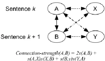
We present in this paper a graph-based represen-tation of documents that models both the long-range scope "influence" of terms and the seman-tic relatedness of terms in a local context. In these graphs, each term is represented by a series of nodes. Each node in the series corresponds to a sentence within the span of that term’s influ-ence, and the weights of the edges are propor-tional to the semantic relatedness among terms in the context. Semantic relatedness between terms is reinforced by the presence of nearby, closely related terms, reflected in increased connection strength between their nodes.
We demonstrate the usefulness of our repre-sentation by applying it to partitioning of docu-ments into topically coherent segdocu-ments. Our segmentation method finds locations in the graph of a document where one group of strongly
con-nected nodes ends and another begins, signaling a shift in topicality. We test this method both on concatenated news articles, and on a more realis-tic segmentation task, closed-captions from commercial television programs, in which topic transitions are more subjective and less distinct. Our methods are unsupervised and require no training; thus they do not require any labeled in-stances of segment boundaries. Our method at-tains results significantly superior to that of Choi (2000), and approaches human performance on segmentation of television closed-captions, where inter-annotator disagreement is high.
2
Graphs of lexical influence
2.1 Summary of the approach
Successful topic segmentation requires some re-presentation of semantic and discourse cohesion, and the ability to detect where such cohesion is weakest. The underlying assumption of segmen-tation algorithms based on lexical chains or other term similarity measures between portions of a document is that continuity in vocabulary reflects topic continuity. Two short examples illustrating topic shifts in television news programs, with accompanying shift in vocabulary, appear in Figure 1.
We model this continuity by first modeling what the extent of a term's influence is. This dif-fers from a lexical chain approach in that we do not model text cohesion through recurrence of terms. Rather, we determine, for each occurrence of a term in the document (excluding terms gen-erally treated as stopwords), what interval of sen-tences surrounding that occurrence is the best estimate of the extent of its relevance. This idea stems from work in Davis, et al. (2004), who describe the use of relevance intervals in multi-media information retrieval. We summarize their procedure for constructing relevance intervals in
section 2.2. Next, we calculate the relatedness of these terms to one another. We use pointwise mutual information (PMI) as a similarity meas-ure between terms, but other measmeas-ures, such as WordNet-based similarity or Wikipedia Miner similarity (Milne and Witten, 2009), could aug-ment or replace it.
S_44 Gatorade has discontinued a drink with his image but that was planned before the company has said and they have issued a statement in support of tiger woods.
S_45 And at t says that while it supports tiger woods personally, it is evaluating their ongoing busi-ness relationship.
S_46 I'm sure, alex, in the near future we're going to see more of this as companies weigh the short term difficulties of staying with tiger woods versus the long term gains of supporting him fully.
S_47 Okay.
S_48 Mark potter, miami.
S_49 Thanks for the wrapup of that.
S_50 We'll go now to deep freeze that's blanketing the great lakes all the way to right here on the east coast.
S_190 We've got to get this addressed and hold down health care costs.
S_191 Senator ron wyden the optimist from oregon, we appreciate your time tonight.
S_192 Thank you.
S_193 Coming up, the final day of free health clinic in kansas city, missouri.
The next step is to construct a graphical repre-sentation of the influence of terms throughout a document. When constructing topically coherent segments, we wish to assess coherence from one sentence to the next. We model similarity be-tween successive sentences as a graph, in which each node represents both a term and a sentence that lies within its influence (that is, a sentence belonging to a relevance interval for that term). For example, if the term ―drink‖ occurs in sen-tence 44, and its relevance interval extends to sentence 47, four nodes will be created for ―drink‖, each corresponding to one sentence in that interval. The edges in the graph connect nodes in successive sentences. The weight of an edge between two terms t and t' consists not only of their relatedness, but is reinforced by the
pres-ence of other nodes in each sentpres-ence associated with terms related to t and t'.
The resulting graph thus consists of cohorts of nodes, one cohort associated with each sentence, and edges connecting nodes in one cohort to those in the next. Edges with a low weight are pruned from the graph. The algorithm for deter-mining topic segment boundaries then seeks lo-cations in which a relatively large number of re-levance intervals for terms with relatively high relatedness end or begin.
In sum, we introduce two innovations here in computing topical coherence. One is that we use the extent of each term's relevance intervals to model the influence of that term, which thus ex-tends beyond the sentences it occurs in. Second, we amplify the semantic relatedness of a term t to a term t' when there are other nearby terms related to t and t'. Related terms thereby rein-force one another in establishing coherence from one sentence to the next.
2.2 Constructing relevance intervals
As noted, the scope of a term's influence is cap-tured through relevance intervals (RIs). We de-scribe here how RIs are created. A corpus—in this case, seven years of New York Times text totaling approximately 325 million words—is run through a part-of-speech tagger. The point-wise mutual information between each pair of terms is computed using a 50-word window.1
PMI values provide a mechanism to measure relatedness between a term and terms occurring in nearby sentences of a document. When processing a document for segmentation, we first calculate RIs for all the terms in that document. An RI for a term t is built sentence-by-sentence, beginning with a sentence where t occurs. A sen-tence immediately succeeding or preceding the sentences already in the RI is added to that RI if it contains terms with sufficiently high PMI val-ues with t. An adjacent sentence is also added to an RI if there is a pronominal believed to refer to t; the algorithm for determining pronominal ref-erence is closely based on Kennedy and Bogu-raev (1996). Expansion of an RI is terminated if there are no motivations for expanding it further. Additional termination conditions can be in-cluded as well. For example, if large local
1
PMI values are constructed for all words other than those
in a list of stopwords. They are also constructed for a li-mited set of about 100,000 frequent multi-word expressions. In our segmentation system, we use only the RIs for nouns and for multiword expressions.bulary shifts or discourse cues signaling the start of end of a section are detected, RIs can be forced to end at those points. In one version of our system, we set these ―hard‖ boundaries using an algorithm based on Choi (2000). In this paper we report segmentation results with and without this limited use of Choi’s algorithm. Lastly, if two RIs for t are sufficiently close (i.e., the end of one lies within 150 words of the start of another), then the two RIs are merged.
The aim of constructing RIs is to determine which portions of a document are relevant to a particular term. While this is related to the goal of finding topically coherent segments, it is of course distinct, as a topic typically is determined by the influence of multiple terms. However, RIs do provide a rough indication of how far a term's influence extends or, put another way, of "smear-ing out" the occurrence of a term over an ex-tended region.
2.3 From relevance intervals to graphs
Consider a sentence Si, and its immediate
succes-sor Si+1. Each of these sentences is contained in
various relevance intervals; let Wi denote the set
of terms with RIs containing Si, and Wi+1 denote
the set containing Si+1.
For each pair of terms a in Wi and b in Wi+1,
we compute a connection strength c(a,b), a non-negative real number that reflects how the two terms are related in the context of Si and Si+1. To
include the context, we take into account that some terms in Si may be closely related, and
should support one another in their connections to terms in Si+1, and vice versa, as suggested
above. Here, we use PMI values between terms as the basis for connection strength, normalized to a similarity score that ranges between 0 and 1, as follows:
The similarity between two terms is set to 0 if this quantity is negative. Also, we assign the maximum value of 1 for self-similarity. We then define connection strength in the following way:
That is, the similarity of another term in Wi or
Wi+1 to b or a respectively, will add to the
con-nection strength between a and b, weighted by the similarity of that term to a or b respectively. Note that this formula also includes in the
sum-mation the similarity s(a,b) between a and b themselves, when either x or y is set to either a or b.2 Figure 2 illustrates this procedure. We nor-malize the connection strength by the total num-ber of pairs in equation (2).
We note in passing that many possible modifi-cations of this formula are easily imagined. One obvious alternative to using the product of two similarity scores is to use the minimum of the two scores. This gives more weight to pair values that are both moderately high, with respect to pairs where one is high and the other low. Apart from this, we could incorporate terms from RIs in sentences beyond these two adjoining sen-tences, we could weight individual terms in Wi or
Wi+1 according to some independent measure of
topical salience, and so on.
Figure 2. Calculation of connection strength be-tween two nodes
What emerges from this procedure is a weighted graph of connections across slices of a document (sentences, in our experiments). Each node in the graph is labeled with a term and a sentence number, and represents a relevance in-terval for that term that includes the indicated sentence. The edges of the graph connect nodes associated with adjacent sentences, and are weighted by the connection strength. Because many weak connections are present in this graph, we remove edges that are unlikely to contribute to establishing topical coherence. There are vari-ous options for pruning: removing edges with connection strengths below a threshold, retaining only the top n edges, cutting the graph between two sentences where the total connection strength of edges connecting the sentences is small, and using an edge betweenness algorithm (e.g., Girvan and Newman, 2002) to remove edges that have high betweenness (and hence are indicative of a "thin" connection).
2 [image:3.595.327.511.301.408.2]
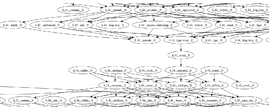
Figure 3. A portion of the graph generated from the first excerpt in Figure 1. Each node is labeled S_i__term_pos, where i indicates the sentence index
We have primarily investigated the first me-thod, removing edges with a connection strength less than 0.5. Two samples of the graphs we pro-duce, corresponding to the excerpts in figure 1, appear in figures 3 and 4.
2.4 Finding segment boundaries in graphs
Segment boundaries in these graphs are hypothe-sized where there are relatively few, relatively weak connections from a cohort of nodes asso-ciated with one sentence to the cohort of nodes associated with the following sentence. If a term has a node in one cohort and in the succeeding cohort (that is, its RI continues across the two corresponding sentences) it counts against a segment boundary at that location, whereas terms with nodes on only one side of the boundary count in favor of a segment. For example, in fig-ure 3, a new set of RIs start in sentence 48, where we see nodes for ―Buffalo‖, ―Michigan‖, ―Worth‖, Marquette‖, and ―Miami‖, and RIs in preceding sentences for ―Tiger Woods‖, ―Gato-rade‖, etc. end. Note that the corresponding ex-cerpt in figure 1 shows a clear topic shift be-tween a story on Tiger Woods ending at sentence 46, and a story about Great Lakes weather be-ginning at sentence 48.
Similarly, in figure 4, RIs for ―Missouri‖, ―city‖ and ―health clinic‖ include sentences 190. 191, and 192; thus these are evidence against a segment boundary at this location. On the other hand, several other terms, such as ―Oregon‖, ―Ron‖, ―Senator‖, and ―bill‖, have RIs that end at sentence 191, which argues in favor of a boundary there. We present further details of our boundary heuristics in section 4.1.
3
Related Work
The literature on topic segmentation has mostly focused on detecting a set of segments, typically non-hierarchical and non-overlapping, exhaus-tively composing a document. Evaluation is then relatively simple, employing pseudo-documents constructed by concatenating a set of documents. This is a suitable technique for detecting coarse-grained topic shifts. As Ferret (2007) points out, approaches to the problem vary both in the kinds of knowledge they depend on, and on the kinds of features they employ.
Figure 4. A portion of the graph generated from the second excerpt in Figure 1. Each node is labeled S_i__term_pos, where i indicates the sentence index
In this respect, our approach also resembles that of Matveeva and Levow (2007), who build semantic similarity among terms into their lexi-cal cohesion model through latent semantic anal-ysis. Our techniques differ in that we incorporate semantic relatedness between terms directly into a graph, rather than computing similarities be-tween blocks of text.
In our experiments, we compare our method to C99 (Choi, 2000), an algorithm widely treated as a baseline. Choi’s algorithm is based on a meas-ure of local coherence; vocabulary similarity be-tween each pair of sentences in a document is computed and the similarity scores of nearby sentences are ranked, with boundaries hypothe-sized where similarity across sentences is low.
4
Experiments, results, and evaluation
4.1 Systems compared
As noted above, we tested our system against the C99 segmentation algorithm (Choi, 2000). The implementation of C99 we use comes from the MorphAdorner website (Burns, 2006). We also compared our system to two simpler baseline systems without RIs. One uses graphs that do not represent a term’s zone of influence, but contain just a single node for each occurrence of a term. The second represents a term’s zone of influence in an extremely simple fashion, as a fixed num-ber of sentences starting from each occurrence of that term. We tried several values ranging from 5 to 20 sentences for this extension. In addition, we varied two parameters to find the best-performing combination of settings: the thre-shold for pruning low-weight edges, and the threshold for positing a segment boundary. In both the single-node and fixed-extension sys-tems, the connection strength between nodes is calculated in the same way as for our full system. These comparisons aim to demonstrate two things. First, segmentation is greatly improved
when we extend the influence of terms beyond the sentences they occur in. Second, the RIs prove more effective than fixed-length exten-sions in modeling that influence accurately.
Lastly, to establish how much we can gain from using Choi’s algorithm to determine termi-nation points for RIs, we also compared two ver-sions of our system: one in which RIs are calcu-lated without information from Choi’s algorithm and a second with these boundaries included.
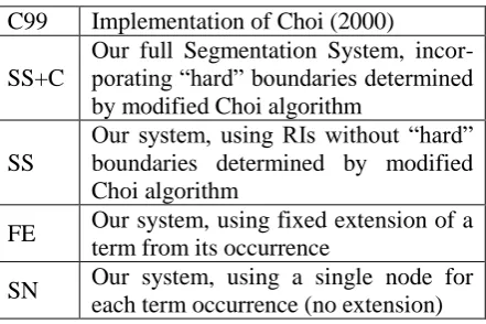
Table 1 lists the systems we compare in the experiments described below.
C99 Implementation of Choi (2000)
SS+C
Our full Segmentation System, incor-porating ―hard‖ boundaries determined by modified Choi algorithm
SS
Our system, using RIs without ―hard‖ boundaries determined by modified Choi algorithm
FE Our system, using fixed extension of a term from its occurrence
SN Our system, using a single node for each term occurrence (no extension)
Table 1. Systems compared in our experiments
4.2 Data and parameter settings
[image:5.595.306.527.407.554.2]interested in our system’s performance on more realistic segmentation tasks, as noted in the in-troduction.
In testing our algorithm, we first generated graphs from the documents in each dataset, as described in section 2. We pruned edges in the graphs with connection strength of less than 0.5. To find segment boundaries, we seek locations where the number of common terms associated with successive sentences is at a minimum. This quantity needs to be normalized by some meas-ure of how many nodes are present on either side of a potential boundary. We tested three normali-zation factors: the total number of nodes on both sides of the potential segment boundary, the maximum of the numbers of nodes on each side of the boundary, and the minimum of the num-bers of nodes on each side of the boundary. The results for all three of these were very similar, so we report only those for the maximum. This measure provides a ranking of all possible boun-daries in a document (that is, between each pair of consecutive sentences), with a value of 0 be-ing most indicative of a boundary. After experi-menting with a few threshold values, we selected a threshold of 0.6, and posit a boundary at each point where the measure falls below this thre-shold.
4.3 Evaluation metrics
We compute precision, recall, and F-measure based on exact boundary matches between the system and the reference segmentation. As nu-merous researchers have pointed out, this alone is not a perspicacious way to evaluate a segmen-tation algorithm, as a system that misses a gold-standard boundary by one sentence would be treated just like one that misses it by ten. We therefore computed two additional, widely used measures, Pk (Beeferman, et al., 1997) and
Win-dowDiff (Pevzner and Hearst, 2002). Pk assesses
a penalty against a system for each position of a sliding window across a document in which the system and the gold standard differ on the pres-ence or abspres-ence of (at least one) segment boun-dary. WindowDiff is similar, but where the sys-tem differs from the gold standard, the penalty is equal to the difference in the number of bounda-ries between the two. This penalizes missed boundaries and ―near-misses‖ less than Pk (but
see Lamprier, et al., (2007) for further analysis and some criticism of WindowDiff). For both Pk
and WindowDiff, we used a window size of half the average reference segment length, as sug-gested by Beeferman, et al. (1997). Pk and
Win-dowDiff values range between 0 and 1, with lower values indicating better performance in detecting segment boundaries. Note that both Pk
and WindowDiff are asymmetrical measures; different values will result if the system’s and the gold-standard’s boundaries are switched.
4.4 Concatenated New York Times articles
The concatenated pseudo-documents consist of New York Times articles selected at random from the New York Times Annotated Corpus.3 Each pseudo-document contains twenty articles, with an average of 623.6 sentences. Our test set con-sists of 185 of these pseudo-documents.4
N = 185
Prec. Rec. F Pk WD
C99 µ 0.404 0.569 0.467 0.338 0.360
s.d 0.106 0.121 0.105 0.109 0.135
SS µ 0.566 0.383 0.448 0.292 0.317
s.d. 0.176 0.135 0.140 0.070 0.084 SS
+C
µ 0.578 0.535 0.537 0.262 0.283
s.d. 0.148 0.197 0.150 0.081 0.098
FE µ 0.265 0.140 0.176 0.478 0.536
s.d. 0.123 0.042 0.055 0.055 0.076
SN µ 0.096 0.112 0.099 0.570 0.702
[image:6.595.299.534.262.419.2]s.d. 0.040 0.024 0.027 0.072 0.164
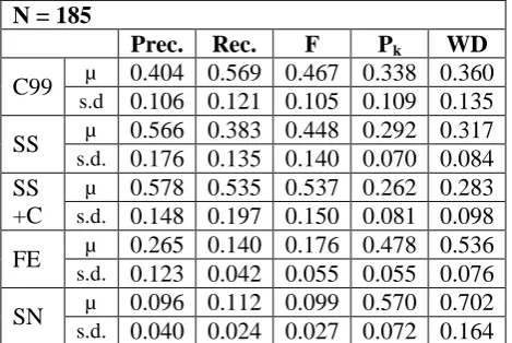
Table 2. Performance of C99 and SS on segmen-tation of concatenated New York Times articles, without specifying a number of boundaries
Tables 2 and 3 provide summary results on the concatenated news articles. We ran the five sys-tems listed in table 1 on the full dataset without any additional restrictions on the number of ar-ticle boundaries to be detected. Means and stan-dard deviations for each method on the five me-trics are displayed in table 2. C99 typically finds many more boundaries than the 20 that are present (30.65 on average). Our SS system finds fewer than the true number of boundaries (14.52 on average), while the combined system SS+C finds almost precisely the correct number (19.98 on average). We used one-tailed paired t-tests of equal means to determine statistical significance at the 0.01 level. Although only SS+C’s perfor-mance is significantly better in terms of
3
www.ldc.upenn.edu/Catalog/CatalogEntry.jsp?catalogId=L DC2008T19
4
measure, both versions of our system outperform C99 according to Pk and WindowDiff.
Using the baseline single node system (SN) yields very poor performance. These results (ta-ble 2, row SN) are obtained with the edge-pruning threshold set to a connection strength of 0.9, and the boundary threshold set to 0.2, at which the average number of boundaries found is 26.86. Modeling the influence of terms beyond the sentences they occur in is obviously valuable. The baseline fixed-length extensions system (FE) does better than SN but significantly worse than RIs. We found that, among the parameter settings yielding between 10 and 30 boundaries per document on average, the best results occur with the extension set to 6 sentences, the edge-pruning threshold set to a connection strength of 0.5, and the boundary threshold set to 0.7. The results for this setting are reported in table 2, row FE (the average number of segments per docu-ment is 12.5). Varying these parameters has only minor effects on performance, although the number of boundaries found can of course be tuned. RIs clearly provide a benefit over this type of system, by modeling a term’s influence dy-namically rather than as a fixed interval.
From here on, we report results only for the two systems: C99 and our best-performing sys-tem, SS+C.
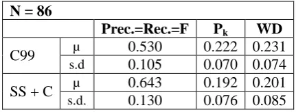
For 86 of the documents, in which both C99 and SS+C found more than 20 boundaries, we also calculate the performance on the best-scoring 20 boundaries found by each system. These results are displayed in table 3. Note that when the number of boundaries to be found by each system is fixed at the actual number of boundaries, the values of precision and recall are necessarily identical. Here too our system out-performs C99, and the differences are statistical-ly significant, according to a one-tailed paired t-test of equal means at the 0.01 level.
N = 86
Prec.=Rec.=F Pk WD
C99 µ 0.530 0.222 0.231
s.d 0.105 0.070 0.074
SS + C µ 0.643 0.192 0.201
[image:7.595.72.288.614.696.2]s.d. 0.130 0.076 0.085
Table 3. Performance of C99 and SS on segmen-tation of concatenated New York Times articles, selecting the 20 best-scoring boundaries
4.5 Human-annotated television program closed-captions
We selected twelve television programs for which we have closed-captions; they are a mix of headline news (3 shows), news commentary (4 shows), documentary/lifestyle (3 shows), one comedy/drama episode, and one talk show. Only the closed captions are used, no speaker intona-tion, video analysis, or metadata is employed. The closed captions are of variable quality, with numerous spelling errors.
Five annotators were instructed to indicate topic boundaries in the closed-caption text files. Their instructions were open-ended in the sense that they were not given any definition of what a topic or a topic shift should be, beyond two short examples, were not told to find a specific number of boundaries, but were allowed to indicate how important a topic was on a five-point scale, en-couraging them to indicate minor segments or subtopics within major topics if they chose to do so. For some television programs, particularly the news shows, major boundaries between sto-ries on disparate topics are likely be broadly agreed on, whereas in much of the remaining material the shifts may be more fine-grained and judgments varied. In addition, the scripted nature of television speech results in many carefully staged transitions and teasers for upcoming ma-terial, making boundaries more diffuse or con-founded than in some other genres.
We combined the five annotators’ segmenta-tions, to produce a single set of boundaries as a reference. We used a three-sentence sliding win-dow, and if three or more of the five annotators place a boundary in that window, we assign a boundary where the majority of them place it (in case of a tie, we choose one location arbitrarily). Although the annotators are rather inconsistent in their use of this rating system, a given annotator tends to be consistent in the granularity of seg-mentation employed across all documents. This observation is consistent with the remarks of Ma-lioutov and Barzilay (2006) regarding varying topic granularity across human annotators on spoken material. We thus computed two versions of the combined boundaries, one in which all boundaries are used, and another in which we ignore minor boundaries—those the annotator assigned a score of 1 or 2. We ran our experi-ments with both versions of the combined boun-daries as the reference segmentation.
We use Pk to assess inter-annotator agreement
Pk values for each pair of annotators; one set of
values is for all boundaries, while the other is for ―major‖ boundaries, assigned an importance of 3 or greater on the five-point scale. The Pk value
for each annotator with respect to the two refer-ence segmentations is also provided.
A B C D E Ref
A 0.36
0.48 0.30 0.45 0.27 0.44 0.42 0.67 0.20 0.38
B 0.29
0.40 0.29 0.32 0.27 0.33 0.33 0.55 0.20 0.25
C 0.57
0.48 0.60 0.44 0.41 0.20 0.67 0.61 0.40 0.18
D 0.36
0.46 0.41 0.46 0.27 0.20 0.53 0.63 0.22 0.26
E 0.33
0.35 0.31 0.34 0.33 0.30 0.32 0.31 0.25 0.27
Ref 0.25
0.39 0.32 0.35 0.24 0.17 0.21 0.22 0.42 0.58
Table 4. Pk values for the segmentations pro-duced by each pair of annotators (A-E) and for the combined annotation described in section 4.5; upper values are for all boundaries and low-er values are for boundaries of segments scored 3 or higher
These numbers are rather high, but compara-ble to those obtained by Malioutov and Barzilay (2006) in a somewhat similar task of segmenting video recordings of physics lectures. The Pk
val-ues are lower for the reference boundary set, which we therefore feel some confidence in us-ing as a reference segmentation.
Prec. Rec. F Pk WD
All topic boundaries
C99 µ 0.197 0.186 0.184 0.476 0.507
s.d 0.070 0.072 0.059 0.078 0.102 SS
+C
µ 0.315 0.208 0.240 0.421 0.462
s.d. 0.089 0.073 0.064 0.072 0.084 Major topic boundaries only
C99 µ 0.170 0.296 0.201 0.637 0.812
s.d. 0.063 0.134 0.060 0.180 0.405 SS
+C
µ 0.271 0.316 0.271 0.463 0.621
s.d. 0.102 0.138 0.077 0.162 0.445
Table 5. Performance of C99 and SS+C on seg-mentation of closed-captions for twelve televi-sion programs, with the two reference segmenta-tions using ―all topic boundaries‖ and ―major topic boundaries only‖
As the television closed-captions are noisy with respect to data quality and inter-annotator disagreement, the performance of both systems is worse than on the concatenated news articles, as expected. We present the summary performance of C99 and SS+C in table 5, again using two ver-sions of the reference. Because of the small test set size, we cannot claim statistical significance for any of these results, but we note that on aver-age SS+C outperforms C99 on all measures.
5
Conclusions and future work
We have presented an approach to text segmen-tation that relies on a novel graph based repre-sentation of document structure and semantics. It successfully models topical coherence using long-range influence of terms and a contextually determined measure of semantic relatedness. Re-levance intervals, calculated using PMI and other criteria, furnish an effective model of a term’s extent of influence for this purpose. Our measure of semantic relatedness reinforces global co-occurrence statistics with local contextual infor-mation, leading to an improved representation of topical coherence. We have demonstrated signif-icantly improved segmentation resulting from this combination, not only on artificially con-structed pseudo-documents, but also on noisy data with more diffuse boundaries, where inter-annotator agreement is fairly low.
Although the system we have described here is not trained in any way, it provides an extensive set of parameters that could be tuned to improve its performance. These include various tech-niques for calculating the similarity between terms and combining those similarities in con-nection strengths, heuristics for scoring potential boundaries, and thresholds for selecting those boundaries. Moreover, the graph representation lends itself to techniques for finding community structure and centrality, which may also prove useful in modeling topics and topic shifts.
We have also begun to explore segment labe-ling, identifying the most ―central‖ terms in a graph according to their connection strengths. Those terms whose nodes are strongly connected to others within a segment appear to be good candidates for segment labels.
Acknowledgements
We thank our colleagues David Houghton, Olivier Jojic, and Robert Rubinoff, as well as the anonymous referees, for their comments and suggestions.
References
Doug Beeferman, Adam Berger, and John Laf-ferty. 1997. Text Segmentation Using Expo-nential Models. Proceedings of the Second Conference on Empirical Methods in Natural Language Processing, 35-46.
Doug Beeferman, Adam Berger, and John Laf-ferty. 1999. Statistical models for text segmen-tation. Machine Learning, 34(1):177–210.
David M. Blei and Pedro J. Moreno. 2001. Topic segmentation with an aspect hidden Markov model. Proceedings of the 24th Annual Meet-ing of ACM SIGIR, 343–348.
Burns, Philip R. 2006. MorphAdorner: Morpho-logical Adorner for English Text. http://morphadorner.northwestern.edu/morpha dorner/textsegmenter/.
Freddy Y.Y. Choi. 2000. Advances in domain independent linear text segmentation. Pro-ceedings of NAACL 2000, 109-117.
Anthony Davis, Phil Rennert, Robert Rubinoff, Tim Sibley, and Evelyne Tzoukermann. 2004. Retrieving what's relevant in audio and video: statistics and linguistics in combination. Pro-ceedings of RIAO 2004, 860-873.
Olivier Ferret. 2007. Finding document topics for improving topic segmentation. Proceedings of the 45th Annual Meeting of the ACL, 480–487.
Michel Galley, Kathleen McKeown, Eric Fosler-Lussier, and Hongyan Jing. 2003. Discourse Segmentation of Multi-Party Conversation. Proceedings of the 41st Annual Meeting of the ACL, 562-569.
Michelle Girvan and M.E.J. Newman. 2002. Community structure in social and biological networks. Proceedings of the National Acad-emy of Sciences, 99:12, 7821-7826.
Marti A. Hearst. 1994. Multi-paragraph segmen-tation of expository text. Proceedings of the 32nd Annual Meeting of the ACL, 9-16.
Marti A. Hearst. 1997. TextTiling: Segmenting Text into Multi-Paragraph Subtopic Passages. Computational Linguistics, 23:1, 33-64.
Min-Yen Kan, Judith L. Klavans, and Kathleen R. McKeown. 1998. Linear Segmentation and Segment Significance. Proceedings of the 6th International Workshop on Very Large Cor-pora, 197-205.
Christopher Kennedy and Branimir Boguraev. 1996. Anaphora for Everyone: Pronominal Anaphora Resolution without a Parser. Pro-ceedings of the 16th International Conference on Computational Linguistics, 113-118.
Hideki Kozima. 1993. Text segmentation based on similarity between words. Proceedings of the 31st Annual Meeting of the ACL (Student Session), 286-288.
Sylvain Lamprier, Tassadit Amghar, Bernard Levrat and Frederic Saubion. 2007. On Evalu-ation Methodologies for Text SegmentEvalu-ation Algorithms. Proceedings of the 19th IEEE In-ternational Conference on Tools with Artifi-cial Intelligence, 19-26.
Igor Malioutov and Regina Barzilay. 2006. Min-imum Cut Model for Spoken Lecture Segmen-tation. Proceedings of the 21st International Conference on Computational Linguistics and 44th Annual Meeting of the ACL, 25–32.
Irina Matveeva and Gina-Anne Levow. 2007. Topic Segmentation with Hybrid Document Indexing. Proceedings of the 2007 Joint Con-ference on Empirical Methods in Natural Language Processing and Computational Natural Language Learning, 351–359,
David Milne and Ian H. Witten. 2009. An Open-Source Toolkit for Mining Wikipedia. http://www.cs.waikato.ac.nz/~dnk2/publicatio ns/AnOpenSourceToolkitForMiningWikipedia .pdf.
Jane Morris and Graeme Hirst. 1991. Lexical cohesion computed by thesaural relations. as an indicator of the structure of text. Computa-tional Linguistics, 17:1, 21-48.