IJEDR1502110
International Journal of Engineering Development and Research (www.ijedr.org)604
Comparative Study for the Effect Powder Mixed
Dielectric on Performance Measures in Wire EDM
Jigar Saliya1, Brijesh K. Gotawala2
1Post Graduate Student, 2Assiatant Professor, Department of Mechanical Engineering, Shri Sa‟d vidyamandal Institute of
Technology, Bharuch, 392001, Gujarat, India
________________________________________________________________________________________________________
Abstract -Requirements of the good surface finish, cost effective ness, intricate geometry, better MRR and minimum overcut have evolved the area of the Advanced Machining processes. Wire EDM is an extended form of Electrical Discharge Machining working on principle of spark erosion. Input parameters of Wire EDM such as Pulse ON time, Pulse Off time, Peak current, wire tension, wire speed etc. have major effect on the performance of the process. Wire cut EDM process is evaluated on the basis of surface finish, MRR, machining time, power consumption and wire erosion. Main emphasis in this research is given to study the effect of PMD (Powder Mixed Dielectric) on optimization results. Use of powder mixed dielectric is the main domain to focus. For experimentation, Taguchi method has been applied to select orthogonal array with using of Minitab 17. To achieve optimized combination of process parameters for best performance, optimization using Grey relational analysis is carried out. Adding the powder in dielectric improve the surface finish and kerf width. In this work, comparative optimization for process parameters of Wire EDM with using simple deionized water and graphite mixed dielectric has been carried out.
Keywords – Wire EDM, Grey Relational analysis, DM water (mineralized water), GMDM water (graphite mixed De-mineralized water)
________________________________________________________________________________________________________
I INTRODUCTION
Wire EDM process was introduced in late 1960‟s and it had revolutionized the tool and die, metal working, mold industries. It is probably the most exciting and diversified machine tool developed for manufacturing industry.It can machine anything that is electrically conductive regardless of the hardness, from relatively common materials such as tool steel, aluminum, copper, and graphite, to exotic space-age alloys including hast alloy, wasp alloy, Inconel, titanium, carbide, polycrystalline diamond compacts and conductive ceramics. It is single step process. Wire electrical-discharge machining is an adaptation of the basic EDM process. In wire EDM process metal removal process is carried out by spark erosion mechanism. When high frequency of alternating or direct current is discharged from wire to work piece with a very small spark gap through dielectric fluid, many sparks can be observed at one time. The heat of each electrical spark, estimated at around15,000° to 21,000° Fahrenheit, erodes away a tiny bit of material that is vaporized and separated from the parent material.The resulting particles (chips) are flushed away from the gap with a stream of clean, de-ionized water from the top and bottom flushing nozzles [1].
Fig. 1 principle of Wire EDM [6]
IJEDR1502110
International Journal of Engineering Development and Research (www.ijedr.org)605
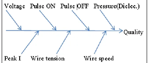
Fig .2 Fishbone diagram showing process parameterII LITERATURE SURVEY
Wire electrical discharge machining (WEDM)
The emphasis is on the generation of mathematical modeling having quadratic nature (respond surface model). Multi-objective optimization with considering discharge current, pulse duration, pulse frequency, wire speed, wire tension and dielectric flow rate as the process parameters are done. Taguchi method with L27 orthogonal array has been selected for experiment and to convert
multi objective criterion to equivalent single objective function grey relational analysis has been adopted. Mathematical model and effects of the highlighted parameters on the performance measures are established with the use of statistical software MINITAB 13 [2]. Optimization of process parameters (peak current, duty factor, wire tension and dielectric pressure) with number of nontraditional optimization techniques (genetic algorithm, particle swarm optimization, sheep flock algorithm, ant colony optimization, artificial bee colony and biogeography-based optimization) is done for wear ratio, surface finish and MRR as performance measures. Among all biogeography based technique provides best results [3]. Prediction and modeling of the surface finish in wire EDM titanium alloy (Ti-6Al-4v) with the use of two levels full factorial method. And experimental values are compared with predicted values. Pulse on time, pulse off time, voltage and dielectric flushing pressure. The WEDM experiments are conducted in Electronica ultra-cut s1 machine using 0.25 mm brass wire as the tool electrode. Comparison between experimental values and predicted values has been carried out and error margin is found to be 7% [4]. Parametric optimization of composite material (Al+3%Sic) with the use of Taguchi method (L13 orthogonal array) is done and compared with
ANNOVA method. Surface finish and MRR decreases when work piece is machined with air as a dielectric fluid [5]. Graphical representation for effect of input parameters on MRR and surface roughness has been carried out and studied using respond surface methodology. Work piece and tool material are SS304 and brass wire. CCD (central composite rotatable factorial design) is adopted as DOE [6]. Mathematical model has been developed using design expert system software and optimization is carried out using MATLAB (GA algorithm). Desired responses are maximum MRR and minimum surface roughness [7]. Mathematical modeling has been done with the use of respond surface modeling with quadratic nature. Pulse on time, pulse of time, wire speed and wire feed are the parameters. Performance measures are MRR and Surface roughness [8]. Wire failure occurred in wire cut EDM is a result of severity in wire wear rate, which is function of discharge current and discharge time. For the same MRR, wire wear rate is observed to be lower with zinc coated brass but with bare wire high erosion rate is observed [9]. WEDM (wire electro discharge grinding) is a one of the hybrid machining process for micro machining the fine electrodes or pins with a large aspect ratio [10].
Use of Powder mixed dielectric in EDM
Electrical conductive powder used in dielectric reduces the insulating strength of dielectric fluid and increases the spark gap between tool & workpiece. It improves MRR and surface finish. Aluminum, chromium, graphite, silicon, copper and silicon carbide are the powders can be used. Powder creates bridging effect [11]. Use of Silicon powder in Wire electro discharge machining has positive influence on the operating time and surface finish and best results are achieved when powder grain size is below 15 µm with AIHI H13 steel [12]. Thin electrode and rotating disk are used to keep powder concentration in gap between workpiece and electrode. TiC layer is grown on carbon steel when titanium powder is used in dielectric [13]. Aluminum powder leads the thinnest rim zone and highest MRR and silicon powder produces grey zone beneath the actual „white zone‟. Powder addition produces the thinner rim zone [14]. With smaller electrode area surface finish is good with simple EDM but with the use of powder mixed dielectric, sensitivity to surface quality is lower. There is linear relationship between electrode area and surface quality [15]. Pick current is emerged as a most significant parameter and tungsten carbide formation in workpiece indicate the reaction of tungsten powder with carbon present in it. Surface alloying with tungsten and carbon has a significant effect on properties of workpiece material [16]. Introduction of the MoS2 micro powder in dielectric fluid using ultrasonic vibration
significantly improves the MRR and surface quality by providing a flat surface free of black carbon spots [17]. Features of powder mixed dielectric EDM are shorter machining time, more uniform dispersion of electrical discharges and stable machining [18].setting of peak current at a high level (16 A), pulse-on time at a medium level (100 μs), pulse-off time at a low level (15 μs), powder concentration at a high level (4 g/l), and gain at a low level (0.83 mm/s) produced optimum MR from AISI D2 surfaces when machined by silicon powder mixed EDM [19]. Pulse on time, duty cycle, peak current and concentration of the silicon powder added into the dielectric fluid of EDM are the variables to study the process performance in terms of material removal rate and surface roughness [20].
IJEDR1502110
International Journal of Engineering Development and Research (www.ijedr.org)606
research. Use of powder mixed dielectric in electrical discharge machining directs the new way of thinking for the improvements. But main gap found is: Comparative study for use of powder mixed dielectric and simple dielectric in Wire EDM process.
Check the effect of concentrations of powder in dielectric on performance measures (surface finish, machining time and kerf width) in Wire EDM.
Use of powder mixed dielectric through nozzle directly.
Use of various mesh sized powder in wire EDM and checking the effect.
Design stirring system for powder mixing in dielectric.
Comparative study for the different types of powders mixed with dielectric in wire EDM process.
Conductive powder addition in dielectric creates “bridging effect” and lowers down the breakdown voltage, which leads early explosion improving MRR. Uniformly distributed sparking in series improves surface roughness. Aluminums, silicon, graphite, are some powder which can be added to enhance the performance of the process. SS304 is a steel material applicable in milk processing equipment and chemical handling due to anti corrosive characteristic against acids. Parametric optimization of wire EDM with simple dielectric on SS304 has been done by previous researcher. But as per literature reviewed, Comparative optimization has not been done for SS304 with PMD use. Hence, for further research it is taken as research gap and accordingly following research objectives has been derived.
1. To experimentally investigate, with the use of Taguchi experimental design, the effect of powder addition (Graphite) on performance characteristics (surface roughness, machining time and kerf width).
2. To carry out grey relation analysis to find optimized combination of control parameters III DESIGN OF EXPERIMENT
Selection of Process parameters, Performance measures, Material and type of Dielectric
Pulse ON time, Pulse OFF time and Peak current are selected as control parameters.
Machining time, kerf width and Surface roughness are taken as quality characteristics.
SS304 is selected as Work piece. Two types of Dielectrics have been selected. First one is, De-mineralized water and second one is Graphite mixed de-mineralized water (Concentration = 2g/litre, fineness = 200 mesh).
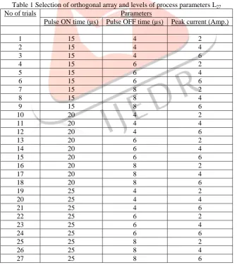
Table 1 Selection of orthogonal array and levels of process parameters L27
No of trials Parameters
Pulse ON time (µs) Pulse OFF time (µs) Peak current (Amp.)
1 15 4 2
2 15 4 4
3 15 4 6
4 15 6 2
5 15 6 4
6 15 6 6
7 15 8 2
8 15 8 4
9 15 8 6
10 20 4 2
11 20 4 4
12 20 4 6
13 20 6 2
14 20 6 4
15 20 6 6
16 20 8 2
17 20 8 4
18 20 8 6
19 25 4 2
20 25 4 4
21 25 4 6
22 25 6 2
23 25 6 4
24 25 6 6
25 25 8 2
26 25 8 4
IJEDR1502110
International Journal of Engineering Development and Research (www.ijedr.org)607
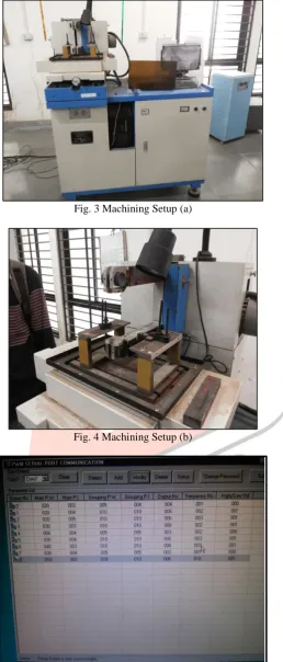
ExperimentationExperiments are performed on the NC controlled Wire Electrical discharge machine (DK – 7712) manufactured by Concord United Pvt. Ltd, Bangalore. It is installed in laboratory of Mechanical Department of Government Engineering College, Patan (N.G)
Table 2 Work table Specifications
Specifications Metric
Longitudinal Travel 160 mm
Transverse Travel 120 mm
Movement of work table per revolution of hand wheel 4 mm Movement of work table per graduation on hand wheel 0.04 mm
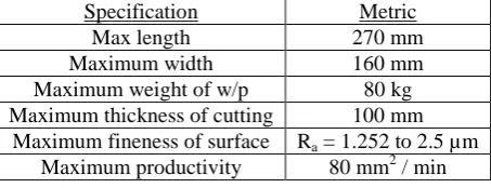
Table 3 Specifications for workpiece handling
Specification Metric
Max length 270 mm
Maximum width 160 mm
Maximum weight of w/p 80 kg Maximum thickness of cutting 100 mm
Maximum fineness of surface Ra = 1.252 to 2.5 µm
Maximum productivity 80 mm2 / min Experimental procedure
Select the work pieces of appropriate dimension. Total no of work pieces are 54, 27 for use of de-ionized water and 27 for use PMD.
Fix the work piece on machine table.
Turn on the computer and open the serial port communication program.
Edit the parameter values of pulse ON time, Pulse OFF time and Peak current as per the combination of experimental trial.
Open the HF control system installed in computer, go in “program” tab then prepare the drawing of profile we want to cut according to the drawing G code is generated. Save the G code file and close the tab.
In HF control system, open another tab “machining”, the go to the “read” and select the program file having G code.
Now, turn ON the machine. Select the “CUT +” tab. Machining will be started according to the prepared program with the movement of table against the wire as a tool.
To retract the tool select “CUT”. When cutting will be finish. Machine will stop..
One cut is made throughout cut along length 25 mm, which is used to measure the surface roughness but one more cut is of approximately 10 mm is made to measure the kerf width.
Whole procedure is done for all nine experimental trials.
Replace the dielectric (de-ionized water) of machine tank with 25 litre of new graphite powder (2g/l) mixed de-ionized water.
Whole procedure is repeated for another nine experimental trials of usage of PMD.
Generally Time is measured by digital watch, but in this experiments time has been calculated by HF control system, it shows the time between cutting starting and end of the programmed cut. In this method of time calculation researcher‟s error does not come in picture.
Surface roughness values are measured by “surface roughness tester” in non-conventional machining laboratory of M.S. University of Baroda. Three readings are taken for each workpiece. Mean value is considered for further work.
Kerf width is measured with the use of “measuring microscope” in metallurgy laboratory of M.S University of Baroda. For accurate measurement, eight readings are taken for each work piece at various points. Mean of them is selected for
IJEDR1502110
International Journal of Engineering Development and Research (www.ijedr.org)608
Fig. 3 Machining Setup (a)Fig. 4 Machining Setup (b)
IJEDR1502110
International Journal of Engineering Development and Research (www.ijedr.org)609
Fig. 6 actual machining of pieceTable 4 Measured Data
For DM water For GMDM water
Ra (µm) Wk (mm) Tm (min) Ra (µm) Wk (mm) Tm (min) 2.06 0.2241 38.25 2.06 0.2223 37.13 2.28 0.2543 18.01 2.31 0.2456 19.11
2.29 0.2741 11.58 2.34 0.2634 12
2.29 0.2223 53.17 1.9 0.2212 53.33 2.58 0.2427 25.39 2.57 0.2412 26.07
3.08 0.2629 16.21 1.97 0.25 16.29
2.06 0.2141 59.22 2.97 0.2123 59.57 2.6 0.2328 32.31 2.68 0.2317 32.36
2.94 0.25 20.43 2.92 0.2456 20.48
2.43 0.2414 36.27 2.39 0.2401 36.44 3.43 0.2619 17.12 3.14 0.2545 18.02
2.54 0.2672 11.51 3.58 0.259 12
1.96 0.2413 47.5 1.92 0.2322 48.17
2.65 0.25 24.25 2.62 0.25 21.35
3.32 0.2671 16.18 3.38 0.259 16.31 1.82 0.2412 59.01 1.77 0.2322 59.51
2.69 0.25 31.48 2.56 0.25 32.02
2.99 0.2586 19.44 2.73 0.259 19.47 2.31 0.2414 35.13 2.45 0.2411 35.28 4.34 0.2686 16.02 3.51 0.2689 16.15 4.42 0.2967 11.06 4.37 0.2918 11.23 2.88 0.2385 49.03 2.53 0.2384 49.2 2.89 0.2675 24.03 2.63 0.2624 24.09 3.39 0.2701 15.08 3.32 0.2719 15.29 2.11 0.2335 55.16 1.93 0.2383 57.26
2.9 0.2578 30.29 2.78 0.253 30.32
3.17 0.2627 19.37 3.05 0.2617 19.48 IV GREY RELATIONAL ANALYSIS
Grey analysis is a new technology used for data analysis. It is also called as grey logic or grey system theory. It is useful in the case of uncertain information. It is particularly applicable in case of little system knowledge.
Grey analysis was invented by professor Deng Julong of Huazhong University of Science and Technology in Wuhan, China. Grey analysis has been successfully used in a wide range of fields diverse as agriculture, ecology, economic planning and forecasting, traffic planning, industrial planning and analysis, management and decision making, irrigation strategy, crop yield forecasting, military affairs, target tracking, population control, communication system design, geology, oil exploration, earthquake prediction, material science, manufacturing, biological protection, environmental impact studies, medical management and the judicial system [21].
Step – 1 Data preprocessing : If the number of experimental trials and number of output parameters (performance measures) is “m” and “n” respectively, then ith trial can be expressed as Y
i = (yi1, yi2, yi3, ……., yin) in decision matrix, where yij is the
IJEDR1502110
International Journal of Engineering Development and Research (www.ijedr.org)610
D = [
] (1)
Decision matrix D can be converted into normality decision matrix D‟. And all yij values are replaced by xij. Hence D‟ can be
expressed as, D‟ = [
] (2)
Normalized values of xij are determined by following equations. There are three types of responses larger the better, smaller the
better and nominal the best.
If the expectancy of response is beneficial type (larger the better), then it can be expressed as Xij = (Yij ˗ min Yij) / (max Yj ˗ min Yj) (3)
If the expectancy of response is non-beneficial type (Smaller the better), then it can be expressed as Xij = (max Yij ˗ Yij) / (max Yj ˗ min Yj) (4)
If the expectancy of response is for target value (nominal the best), then it can be expressed as Xij = 1–[(Yj* ˗ Yij) / (max Yij ˗ min Yij)] (5)
Where Yj* is the closer to the desired value of response.
Step 2 Reference sequence definition: All the values of normalized matrix D‟ are in [0,1]. Now, if any xij values are equal to 1
or nearer to 1, then performance of their respective experiment is best for respective response. Reference sequence X is defined as (x1, x2,….xj, ……..xn) = (1, 1, 1, ……., 1). Where, xj is the reference value for jth response. It is used to find experiment whose
comparability sequence is nearest to the reference sequence.
Step 3 Grey relational coefficient calculations: Grey relational coefficient is applicable to show the closeness of xij to xj. As
larger the coefficient value, more is the closeness of xij to xj. Coefficients can be expressed as
ᵞij=
(6)
For i = 1, 2, 3….,m and j = 1, 2, 3,….n
Where,ᵞ = grey relational grade between xij and xj.
| | (7)
| | (8)
| | (9)
ξ = distinguishing coefficient ξ ϵ (0, 1)
Distinguishing coefficient is also called as index for distinguishing ability. It represents the “contrast control” of equation. Smaller the value of coefficient, higher is the distinguishing ability. Application of this coefficient is to expend or compress the range of grey relational coefficient. Different values can give different values. Here, we take value ξ = 0.4.
Step 4 Calculation of grey relational grades (grey relational degree): It is a weighted sum of grey relational coefficients. It can be calculated using following equation,
ᵞj=∑ (10)
For i = 1, 2…, m. and j = 1, 2…, n.
ᵞjis the grey relational grade between comparability sequence and reference sequence.
Wj is the Weightage factor for particular response j and it depends on priorities of researcher.
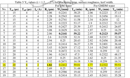
Table 5 Yij values (i = 1,2,….,27) for Machining time, surface roughness, kerf width.
For DM water For GMDM water
No. Ton (µs) Toff (µs) Ip (A) Ra (µm) Wk (mm) Tm (min) Ra (µm) Wk (mm) Tm (min)
1 15 4 2 2.06 0.2241 38.25 2.06 0.2223 37.13
2 15 4 4 2.28 0.2543 18.01 2.31 0.2456 19.11
3 15 4 6 2.29 0.2741 11.58 2.34 0.2634 12
4 15 6 2 2.29 0.2223 53.17 1.9 0.2212 53.33
5 15 6 4 2.58 0.2427 25.39 2.57 0.2412 26.07
6 15 6 6 3.08 0.2629 16.21 1.97 0.25 16.29
7 15 8 2 2.06 0.2141 59.22 2.97 0.2123 59.57
8 15 8 4 2.6 0.2328 32.31 2.68 0.2317 32.36
9 15 8 6 2.94 0.25 20.43 2.92 0.2456 20.48
10 20 4 2 2.43 0.2414 36.27 2.39 0.2401 36.44
11 20 4 4 3.43 0.2619 17.12 3.14 0.2545 18.02
12 20 4 6 2.54 0.2672 11.51 3.58 0.259 12
13 20 6 2 1.96 0.2413 47.5 1.92 0.2322 48.17
14 20 6 4 2.65 0.25 24.25 2.62 0.25 21.35
15 20 6 6 3.32 0.2671 16.18 3.38 0.259 16.31
16 20 8 2 1.82 0.2412 59.01 1.77 0.2322 59.51
17 20 8 4 2.69 0.25 31.48 2.56 0.25 32.02
18 20 8 6 2.99 0.2586 19.44 2.73 0.259 19.47
IJEDR1502110
International Journal of Engineering Development and Research (www.ijedr.org)611
20 25 4 4 4.34 0.2686 16.02 3.51 0.2689 16.15
21 25 4 6 4.42 0.2967 11.06 4.37 0.2918 11.23
22 25 6 2 2.88 0.2385 49.03 2.53 0.2384 49.2
23 25 6 4 2.89 0.2675 24.03 2.63 0.2624 24.09
24 25 6 6 3.39 0.2701 15.08 3.32 0.2719 15.29
25 25 8 2 2.11 0.2335 55.16 1.93 0.2383 57.26
26 25 8 4 2.9 0.2578 30.29 2.78 0.253 30.32
27 25 8 6 3.17 0.2627 19.37 3.05 0.2617 19.48
Max 4.42 0.2967 59.22 4.37 0.2918 59.57
Min 1.82 0.2141 11.06 1.77 0.2123 11.23
Max - Min 2.6 0.0826 48.16 2.6 0.0795 48.34
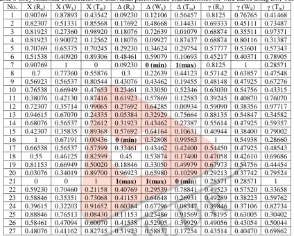
Table 6 Sequence of each performance measures after data processing for wire EDM with DM water No. X (Ra) X (Wk) X (Tm) Δ (Ra) Δ (Wk) Δ (Tm)
1 0.90769 0.87893 0.43542 0.09230 0.12106 0.56457 2 0.82307 0.51331 0.85568 0.17692 0.48668 0.14431 3 0.81923 0.27360 0.98920 0.18076 0.72639 0.01079 4 0.81923 0.90072 0.12562 0.18076 0.09927 0.87437 5 0.70769 0.65375 0.70245 0.29230 0.34624 0.29754 6 0.51538 0.40920 0.89306 0.48461 0.59079 0.10693 7 0.90769 1 0 0.09230 0 (min) 1(max) 8 0.7 0.77360 0.55876 0.3 0.22639 0.44123 9 0.56923 0.56537 0.80544 0.43076 0.43462 0.19455 10 0.76538 0.66949 0.47653 0.23461 0.33050 0.52346 11 0.38076 0.42130 0.87416 0.61923 0.57869 0.12583 12 0.72307 0.35714 0.99065 0.27692 0.64285 0.00934 13 0.94615 0.67070 0.24335 0.05384 0.32929 0.75664 14 0.68076 0.56537 0.72612 0.31923 0.43462 0.27387 15 0.42307 0.35835 0.89368 0.57692 0.64164 0.10631 16 1 0.67191 0.00436 0 (min) 0.32808 0.99563 17 0.66538 0.56537 0.57599 0.33461 0.43462 0.42400 18 0.55 0.46125 0.82599 0.45 0.53874 0.17400 19 0.81153 0.66949 0.50020 0.18846 0.33050 0.49979 20 0.03076 0.34019 0.89700 0.96923 0.65980 0.10299
21 0 0 1 1(max) 1(msx) 0 (min)
22 0.59230 0.70460 0.21158 0.40769 0.29539 0.78841 23 0.58846 0.35351 0.73068 0.41153 0.64648 0.26931 24 0.39615 0.32203 0.91652 0.60384 0.67796 0.08347 25 0.88846 0.76513 0.08430 0.11153 0.23486 0.91569 26 0.58461 0.47094 0.60070 0.41538 0.52905 0.39929 27 0.48076 0.41162 0.82745 0.51923 0.58837 0.17254
Table 7 Sequence of each performance measures after data processing for wire EDM with GMDM water No. X (Ra) X (Wk) X (Tm) Δ (Ra) Δ (Wk) Δ (Tm)
IJEDR1502110
International Journal of Engineering Development and Research (www.ijedr.org)612
18 0.63076 0.41257 0.82954 0.36923 0.58742 0.1704519 0.73846 0.63773 0.50248 0.26153 0.36226 0.49751 20 0.33076 0.28805 0.89822 0.66923 0.71194 0.10177
21 0 0 1 1(max) 1(max) 0(min)
22 0.70769 0.67169 0.21452 0.29230 0.32830 0.78547 23 0.66923 0.36981 0.73396 0.33076 0.63018 0.26603 24 0.40384 0.25031 0.91601 0.59615 0.74968 0.08398 25 0.93846 0.67295 0.04778 0.06153 0.32704 0.95221 26 0.61153 0.48805 0.60508 0.38846 0.51194 0.39491 27 0.50769 0.37861 0.82933 0.49230 0.62138 0.17066
Table 8 Grey relational coefficients for individual performance characteristics for wire EDM using DM water No. X (Ra) X (Wk) X (Tm) Δ (Ra) Δ (Wk) Δ (Tm) γ (Ra) γ (Wk) γ (Tm)
1 0.90769 0.87893 0.43542 0.09230 0.12106 0.56457 0.8125 0.76765 0.41468 2 0.82307 0.51331 0.85568 0.17692 0.48668 0.14431 0.69333 0.45111 0.73487 3 0.81923 0.27360 0.98920 0.18076 0.72639 0.01079 0.68874 0.35511 0.97371 4 0.81923 0.90072 0.12562 0.18076 0.09927 0.87437 0.68874 0.80116 0.31387 5 0.70769 0.65375 0.70245 0.29230 0.34624 0.29754 0.57777 0.53601 0.57343 6 0.51538 0.40920 0.89306 0.48461 0.59079 0.10693 0.45217 0.40371 0.78905 7 0.90769 1 0 0.09230 0 (min) 1(max) 0.8125 1 0.28571 8 0.7 0.77360 0.55876 0.3 0.22639 0.44123 0.57142 0.63857 0.47548 9 0.56923 0.56537 0.80544 0.43076 0.43462 0.19455 0.48148 0.47925 0.67276 10 0.76538 0.66949 0.47653 0.23461 0.33050 0.52346 0.63030 0.54756 0.43315 11 0.38076 0.42130 0.87416 0.61923 0.57869 0.12583 0.39245 0.40870 0.76070 12 0.72307 0.35714 0.99065 0.27692 0.64285 0.00934 0.59090 0.38356 0.97717 13 0.94615 0.67070 0.24335 0.05384 0.32929 0.75664 0.88135 0.54847 0.34582 14 0.68076 0.56537 0.72612 0.31923 0.43462 0.27387 0.55614 0.47925 0.59357 15 0.42307 0.35835 0.89368 0.57692 0.64164 0.10631 0.40944 0.38400 0.79002 16 1 0.67191 0.00436 0 (min) 0.32808 0.99563 1 0.54938 0.28660 17 0.66538 0.56537 0.57599 0.33461 0.43462 0.42400 0.54450 0.47925 0.48543 18 0.55 0.46125 0.82599 0.45 0.53874 0.17400 0.47058 0.42610 0.69686 19 0.81153 0.66949 0.50020 0.18846 0.33050 0.49979 0.67973 0.54756 0.44454 20 0.03076 0.34019 0.89700 0.96923 0.65980 0.10299 0.29213 0.37742 0.79524 21 0 0 1 1(max) 1(max) 0 (min) 0.28571 0.28571 1 22 0.59230 0.70460 0.21158 0.40769 0.29539 0.78841 0.49523 0.57520 0.33658 23 0.58846 0.35351 0.73068 0.41153 0.64648 0.26931 0.49289 0.38223 0.59762 24 0.39615 0.32203 0.91652 0.60384 0.67796 0.08347 0.39846 0.37106 0.82734 25 0.88846 0.76513 0.08430 0.11153 0.23486 0.91569 0.78195 0.63005 0.30402 26 0.58461 0.47094 0.60070 0.41538 0.52905 0.39929 0.49056 0.43054 0.50044 27 0.48076 0.41162 0.82745 0.51923 0.58837 0.17254 0.43514 0.40470 0.69862
Table 9 Grey relational coefficients for individual performance characteristics for wire EDM using GMDM water No. X (Ra) X (Wk) X (Tm) Δ (Ra) Δ (Wk) Δ (Tm) γ (Ra) γ (Wk) γ (Tm)
IJEDR1502110
International Journal of Engineering Development and Research (www.ijedr.org)613
19 0.73846 0.63773 0.50248 0.26153 0.36226 0.49751 0.60465 0.52475 0.4456720 0.33076 0.28805 0.89822 0.66923 0.71194 0.10177 0.37410 0.35972 0.79716
21 0 0 1 1(max) 1(max) 0(min) 0.28571 0.28571 1
22 0.70769 0.67169 0.21452 0.29230 0.32830 0.78547 0.57777 0.54922 0.33741 23 0.66923 0.36981 0.73396 0.33076 0.63018 0.26603 0.54736 0.38827 0.60057 24 0.40384 0.25031 0.91601 0.59615 0.74968 0.08398 0.40154 0.34792 0.82646 25 0.93846 0.67295 0.04778 0.06153 0.32704 0.95221 0.86666 0.55017 0.29581 26 0.61153 0.48805 0.60508 0.38846 0.51194 0.39491 0.50731 0.43862 0.50320 27 0.50769 0.37861 0.82933 0.49230 0.62138 0.17066 0.44827 0.39162 0.70093
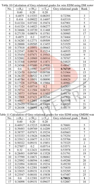
Table 10 Calculation of Grey relational grades for wire EDM using DM water No. γ (Ra) γ (Wk) γ (Tm) Grey relational grade Rank
0.60 0.20 0.20
1 0.4875 0.15353 0.08293 0.72396 3
2 0.416 0.09022 0.14697 0.65319 7
3 0.41324 0.07102 0.19474 0.67901 5 4 0.41324 0.16023 0.06277 0.63625 8 5 0.34666 0.10720 0.11468 0.56855 12 6 0.27130 0.08074 0.15781 0.50985 17
7 0.4875 0.2 0.05714 0.74464 2
8 0.34285 0.12771 0.09509 0.56567 13 9 0.28888 0.09585 0.13455 0.51929 16 10 0.37818 0.10951 0.08663 0.57432 11 11 0.23547 0.08174 0.15214 0.46935 25 12 0.35454 0.07671 0.19543 0.62669 9 13 0.52881 0.10969 0.06916 0.70767 4 14 0.33368 0.09585 0.11871 0.54825 14 15 0.24566 0.07680 0.15800 0.48047 22
16 0.6 0.10987 0.05732 0.76719 1
17 0.32670 0.09585 0.09708 0.51964 15 18 0.28235 0.08522 0.13937 0.50694 18 19 0.40784 0.10951 0.08890 0.60626 10 20 0.17528 0.07548 0.15904 0.40981 27
21 0.17142 0.05714 0.2 0.42857 26
22 0.29714 0.11504 0.06731 0.47950 23 23 0.29573 0.07644 0.11952 0.49170 19 24 0.23908 0.07421 0.16546 0.47876 24 25 0.46917 0.12601 0.06080 0.65598 6 26 0.29433 0.08610 0.10008 0.48053 21 27 0.26108 0.08094 0.13972 0.48175 20
Table 11 Calculation of Grey relational grades for wire EDM using GMDM water No. γ (Ra) γ (Wk) γ (Tm) Grey relational grade Rank
0.60 0.20 0.20
1 0.46917 0.15215 0.08548 0.70681 5 2 0.39493 0.09769 0.14209 0.63472 8 3 0.38757 0.07671 0.19234 0.65663 7 4 0.53333 0.15626 0.06294 0.75254 3 5 0.33913 0.10477 0.11315 0.55706 10 6 0.50322 0.09151 0.15851 0.75325 2
7 0.27857 0.2 0.05714 0.53571 14
8 0.32 0.12421 0.09556 0.53978 13
9 0.28493 0.09769 0.13528 0.51791 19 10 0.37590 0.10671 0.08681 0.56942 9 11 0.25892 0.08594 0.14802 0.49288 20 12 0.21894 0.08101 0.19234 0.49230 22 13 0.52436 0.12301 0.06871 0.71610 4 14 0.33015 0.09151 0.13128 0.55295 12 15 0.23547 0.08101 0.15838 0.47487 25
16 0.6 0.12301 0.05719 0.78021 1
IJEDR1502110
International Journal of Engineering Development and Research (www.ijedr.org)614
18 0.312 0.08101 0.14023 0.53325 1519 0.36279 0.10495 0.08913 0.55687 11 20 0.22446 0.07194 0.15943 0.45583 26
21 0.17142 0.05714 0.2 0.42857 27
22 0.34666 0.10984 0.06748 0.52399 18 23 0.32842 0.07765 0.12011 0.52619 17 24 0.24092 0.06958 0.16529 0.47580 24
25 0.52 0.11003 0.05916 0.68919 6
26 0.30439 0.08772 0.10064 0.49275 21 27 0.26896 0.07832 0.14018 0.48747 23 Optimization Results
Table 10 and 11 show the grey relational grades and rankings for Wire EDM with simple DM water and GMDM water respectively. From both tables it can be observed that, DOE serial 16th is an optimized combination of parameter for both cases (0.76719 and 0.78021 grades respectively).
Experimentally it is observed that, use of powder mixed Dielectric (Graphite) gives better performance with Optimized combination of parameters (DOE serial 16) than simple dielectric usage. There is a matching in experimental findings and optimized result showing improvement insurface finish and kerf width with larger pulse ON time and pulse off time.
It is observed that, ξ = 0.40 and weight factor (0.6,0.2 and 0.4 for SR, kerf and machining time respectively, give optimization result (pulse on time = 40 sec, pulse off time = 4 sec, peak current = 2 amp).
V CONCLUSION
Graphite powder addition with 2g/litre concentration in dielectric has positive effect on surface roughness and kerf width but negative effect on Machining time.
Optimization of both cases give 16th combination of parameter (Pulse On time = 20 µs, Pulse off time = 4 µs, peak current = 2 A) considering ξ = 0.4 for best performance.
In surface roughness and kerf width optimum parameter combination gives improved value (2.74 % decrement) and (3.73 % decrement) respectively due to graphite powder mixing in simple DM water. But in contrast, for machining time optimum parameter combination gives more value (0.84% increment).
REFERENCES
[1] Donald B. Moulton, “Wire EDM, The Fundamental.
[2] Saurav Datta1, SibaSankarMahapatra, 2010, “Modeling, simulation and parametric optimization of wire EDM process using response surface methodology coupled with grey-Taguchi technique.”, International Journal of Engineering, Science and Technology, Vol. 2, No. 5, pp. 162-183.
[3] Rajarshi Mukherjee, Shankar Chakraborty, SumanSamanta, 2012, “Selection of Wire electrical Discharge Machining processs parameters using nontraditional optimization algorithm”, Applied Soft Computing, Vol. 12, Issue 8, pp. 2506-2516.
[4] Basil Kuriachen, Dr. Josephkunju Paul, Dr.Jose Mathew, 2012, “Modeling of Wire Electrical Discharge Machining Parameters Using Titanium Alloy (Ti-6AL-4V)”, International Journal of Emerging Technology and Advanced Engineering, Vol. 2, Issue 4, pp 377-381.
[5] Sateesh Kumar Reddy K,Ramesh S, 2012, “Parametric Optimization of Wire Electrical Discharge Machining of Composite Material”, International Journal of Advanced Research in Computer Engineering & Technology Vol. 1, Issue 3.
[6] M.Geetha, BezawadaSreenivasulu, G. HarinathGowd, 2013, “Modeling & Analysis of performancecharacteristics of Wire EDM of SS304”, International Journal of Innovative Technology and Exploring Engineering, Vol. 3.
[7] Rajneesh Kumar Singh, D.K. Singh, 2013, “Control parameters optimization of wire – EDM by using Genetic Algorithm”, VSRD International Journal of Mechanical, Civil, Automobile and Production Engineering, Vol. III, Issue IX, pp. 327-332.
[8] K. Kumar, R. Ravikumar, 2013, “Modeling and Optimization of Wire EDM Process”, International Journal of Modern Engineering Research, Vol. 3, Issue. 3, pp. 1645-1648.
[9] B.J.Ranganath, K.G.Sudhakar, A.S.Srikantappa, 2013, “Wire Failure Analysis in Wire-EDM Process”, International Conference on Mechanical Engineering.
[10] K.H Ho, S.T Newman, S. Rahimfard, R.D Allen, 2004, “State of art in Wire electrical discharge machining (WEDM)”,
International Journal of Machine Tools and
[11] Manufacture”, Vol. 44, Issue. 12-13, pp. 1247-1259.
[12] H.K. Kansal, Sehijpal Singh, Pradeep Kumar, 2007, “Technology and Research developments in powder mixed dielectric discharge machining (PMEDM)”, Journal of Material Processing Technology, Vol. 184, Issue 1-3, pp. 32-41. [13] P Peças, E Henriques, 2003, “Influence of silicon powder-mixed dielectric on conventional electrical discharge
machining”, International Journal of Machine Tools and Manufacture, Vol. 43, Issue. 14, pp. 1465-1471.
IJEDR1502110
International Journal of Engineering Development and Research (www.ijedr.org)615
[15] F.Klocke, D. lung et al, 2004, “The effect of powder suspended dielectrics on thermal influenced Zone by electrodischarge machining with small discharge energies”, Journal of Material Processing Technology, Vol. 149, Issue 1-3, pp. 191-197.
[16] P. Pecas, E. Henriques, 2008, “Electrical discharge machining using simple and powder dielectric- The effect of electrode area in Surface and Topography”, Journal of material processing Technology, Vol. 200, Issue 1-3, pp. 250-258.
[17] Sanjeev Kumar, Uma Batra, 2012, “Surface modification of Die steel materials by EDM method Using tungsten powder mixed dielectric”, Jounal of Manufacturing process, Vol. 44, Issue 12-13, pp. 1247-1259.
[18] GunawansetiaPrihandana et al, 2009, “Effect of micro powder suspension and ultrasonic vibration of dielectric fluid in Micro EDM process- Taguchi Approach”, International journal of Machine tools and manufacture, Vol. 49, Issue 12-13, pp. 1035-1041.
[19] Y.S. Weng, L.C. Lim, IqbalRahuman, W.M Tee, 1998, “Near-mirror finish phenomenon in EDM using powder mixed dielectric”, Journal of Material processing Technology, Vol. 79, Issue 1-3, pp. 30-40.
[20] H.K. Kansal, Sehijpal Singh, Pradeep Kumar, 2007, “Effect of Silicon Powder Mixed EDM on Machining Rate of AISI D2 Die Steel”, Journal of Manufacturing Processes, Vol. 9, Issue 1, pp. 13-22.
[21] H.K. Kansal, Sehijpal Singh, Pradeep Kumar, 2005, “Parametric optimization of powder mixed electrical discharge machining by response surface methodology”, Journal of Materials Processing Technology, Vol. 169, Issue 3, pp. 427-436.
![Fig. 1 principle of Wire EDM [6]](https://thumb-us.123doks.com/thumbv2/123dok_us/8402324.1386111/1.595.175.421.501.703/fig-principle-of-wire-edm.webp)