Diffusion tensor echo planar imaging with high spatial resolution and its applications

(1)

D iffusion Tensor Echo Planar Im aging w ith

H igh Spatial R eso lu tio n and Its

A p p lication s

Jiun-Jie Wang

Department of Medical Physics and Bioengineering University College London

Submitted as a Ph.D. Thesis

(2)

ProQuest Number: 10015794

INFORMATION TO ALL USERS

The quality of this reproduction is dependent upon the quality of the copy submitted.

In the unlikely event that the author did not send a complete manuscript and there are missing pages, these will be noted. Also, if material had to be removed,

a note will indicate the deletion.

uest.

ProQuest 10015794

Published by ProQuest LLC(2016). Copyright of the Dissertation is held by the Author.

This work is protected against unauthorized copying under Title 17, United States Code. Microform Edition © ProQuest LLC.

ProQuest LLC

789 East Eisenhower Parkway P.O. Box 1346

(3)

(4)

C on ten ts

1 Introduction 15

1.1 Applications of Diffusion Imaging in Human B ra in ... 15

1.2 Overview of the T h e s is ... 17

2 Diffusion W eighted Echo Planar Imaging 19 2.1 General Introduction to MRl ... 19

2.2 k-space... 20

2.2.1 Image R e so lu tio n ... 20

2.3 Echo Planar Im a g in g ... 21

2.3.1 Historical B a c k g ro u n d ... 21

2.3.2 Image Acquisition and Reconstruction in E P l ... 22

2.3.3 Hardware D e m a n d ... 25

2.4 Diffusion Weighted M R l ... 27

2.4.1 History of Diffusion Weighted M R l ... 27

(5)

CONTENTS

2.4.3 Einstein E q u atio n ... 29

2.4.4 Measuring Diffusion with M R l... 30

2.4.5 Choosing the b-factor... 33

2.5 Diffusion Tensor Im aging... 35

2.5.1 Diffusion Anisotropy in Human Environm ent... 37

2.5.2 Introduction to the Diffusion Tensor ... 38

2.5.3 Definition of b-matrix ... 38

2.5.4 Display of the Diffusion T e n s o r ... 39

2.5.5 Trace of the Diffusion Tensor ... 41

2.5.6 Characterising Diffusion A nisotropy... 42

2.6 Protocols in Measuring the Diffusion T e n s o r ... 46

3 Single Shot Diffusion Tensor EPI 49 3.1 Phantom S t u d y ... 50

3.2 Study on Healthy V olunteers... 50

3.3 Study on A Stroke P a t ie n t... 58

4 Diffusion Tensor E PI w ith High Spatial R esolution 64 4.1 Development of 2D Interleaved E P I ... 65

4.2 Development of EPI Sequences with Half Fourier A cquisition... 68

4.3 Ghost in EPI and Its C orrection... 69

(6)

CONTENTS

4.3.2 Sources of the G h o s t ... 76

4.3.3 Three Navigator Echoes C o rrec tio n ... 79

4.4 Signal-to-Noise R a ti o ... 80

4.4.1 Definition of S N R ... 80

4.4.2 Effects of Low S N R ... 82

4.4.3 Comparison of SNRs from Various Sequences ... 84

5 Selective A veraging 92 5.1 Data Acquisition and T h resh o ld in g ... 93

5.1.1 Data Acquisition with Interleaved E P I ... 93

5.1.2 Thresholding ... 94

5.2 Selective Averaging A lg o rith m s... 94

5.3 A Phantom S tu d y ... 95

5.4 Study on the Human V o lu n te e r... 97

5.5 D iscussion... 98

5.6 Conclusion...104

6 Half-FOV D T -E P I 105 6.1 Phase Variations in the Interleaved EPI S e q u e n c e ... 105

6.2 Sequence of Half-FOV E P I ... 106

6.3 Study on the Phantom with Half-FOV D T - E P I ... 109

(7)

CONTENTS

7 D T -E P I w ith High Spatial R esolution 116

7.1 Methods and M a te r ia l ...116

7.2 Result from C o m p ariso n ...117

7.2.1 Signal-to-Noise R a tio ... 117

7.2.2 Apparent Diffusion Coefficient... 121

7.2.3 T race... 121

7.2.4 Fractional Anisotropy... 121

7.3 D iscussion...124

7.3.1 Acquisition S p e e d ... 124

7.3.2 S N R ... 127

7.3.3 T race... 128

7.3.4 Fractional Anisotropy... 129

8 N euron Fiber Tracking W ith the Diffusion Tensor 134 8.1 Introduction to white matter fiber trac k in g ...134

8.2 Method and T heory... 138

8.2.1 Diffusion Tensor Data Used in the Fiber T ra c k in g ...138

8.2.2 Fiber Tracking A lg o rith m ...140

8.3 Fiber Tracking in the Genu of the Corpus C allo su m ... 141

(8)

CONTENTS

8.3.2 Trajectory in Anisotropic Voxels...143

8.4 D iscussion...147

9 Conclusion 150

(9)

List o f F igures

2.1 Gradient Timing Diagram of An Echo Planar Imaging S eq u en ce... 23

2.2 Structure of a Typical Spin Echo Diffusion Weighted EPI Sequence . . . 31

2.3 Optimization of B-Factor Over a Range of Tg and ADC V alues... 36 2.4 The Diffusion Tensor Displayed as Ellipsoids in an Enlarged ROI . . . . 41

2.5 The Trace And Three Eigen Images of the Diffusion Tensor ... 43

2.6 Maps of Fractional Anisotropy and Relative Anisotropy in a Human Brain 45

3.1 The Trace Images and the Eigenimages of the Doped Phantom Acquired with the Single Shot DT-EPI Sequences ... 52

3.2 The Fractional Anisotropy Map of the Phantom Acquired with the Single Shot EPI Sequences... 53

3.3 The Calculated Trace/3 from Three ROIs in Six Subjects from Two Mea surements ... 56

3.4 The Calculated Fractional Anisotropy from Three ROIs in Six Subjects from Two M easurem ents... 57

(10)

LIST OF FIGURES

3.6 Images of Fractional Anisotropy and Trace from a Stroke Patient 4 Weeks

After the I n s u l t ... 61

3.7 Images of Fractional Anisotropy and Trace from a Stroke Patient 21 Weeks After the I n s u l t ... 62

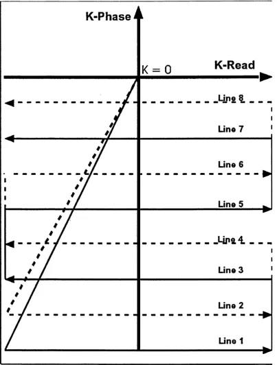
4.1 The K-Space Acquisition Order of the 2D Interleaved EPI Sequence . . . 66

4.2 Brain Images Acquired by the 2D Interleaved EPI S e q u e n c e ... 67

4.3 Brain Images Acquired by the HF-EPI Sequence... 70

4.4 Image of the Simulated Phantom for Ghost L o c a tio n ... 72

4.5 Image of the Phantom with Ghost at Position of Half the Field of View . 73 4.6 Image of the Phantom with Ghost at Position of Quarter the Field of View 74 4.7 Image of Phantom with Ghosts from Various S o u rc e s ... 75

4.8 An EPI Sequence with Two 180 Degree RF P u lses... 78

4.9 Images Showing the Improvement from the Phase Correction by Three Navigator E c h o e s ... 80

4.10 Effect of SNR on DTI in a Phantom ... 85

4.11 Effect of SNR on the measurement of the T r a c e ... 86

4.12 Effect of SNR on Fractional A nisotropy... 87

5.1 The Trace Images and the Measured ADG of the Gel Phantom with Se lective A v e ra g in g ... 96

(11)

LIST OF FIGURES

5.4 Intensity of the Ghost Relative to the Signal For Complex Averages . . . 102

5.5 The Trace Image Computed from Both Averaging A lg o rith m s ... 103

6.1 Diagram Visualizing the Acquisition Process of the Half-FOV EPI Sequence 107 6.2 Slice Profile After the Application of Saturation P u ls e ... 108

6.3 Brain Images Acquired W ith the Half-FOV EPI S eq u en ces...I l l 6.4 Trace Images Of the Brain Acquired with the Half-FOV EPI Sequences . 112 6.5 Fractional Anisotropy Map Acquired W ith the Half-FOV EPI Sequences 113 7.1 SNR Measured in DT-EPI Sequences C om parison... 120

7.2 Images of the Diffusion Coefficients from Sequences in Comparison . . . . 122

7.3 The Trace Image from One Subject Measured by Sequences in DT-EPI C o m p ariso n ...123

7.4 Fractional Anisotropy Map of One Subject Measured by Sequences in DT-EPI C o m p ariso n ... 125

7.5 Recorded ECC Curve From a Human V o lu n teer... 127

7.6 Subtraction Image of the T r a c e ... 130

7.7 Subtraction Image of the Fractional A n iso tro p y ... 132

8.1 Quiver Map of an ROI in the Corpus Callosum ... 136

8.2 Trajectory in the Cenu of the Corpus Callosum from the Data Acquired in Single Session...142

(12)

LIST OF FIGURES 10

8.4 Trajectory in the Genu of the Corpus Callosum for Different Slice Thickness 145

(13)

List o f Tables

2.1 Standard Diffusion Encoding S c h e m e ... 47

2.2 Tetrahedral Diffusion Encoding Schem e... 48

3.1 Diffusion Tensor, Trace and Fractional Anisotropy from a Doped Phantom 51

3.2 Diffusion Measurements from ROIs in Six Healthy Volunteers... 55 3.3 Differences in the Diffusion Parameters Measured from Two Independent

A cquisitions... 58

3.4 Trace and Fractional Anisotropy Measured from the Stroke Patient . . . 60

4.1 Effect of SNR on the Measurement of Diffusion P r o p e r tie s ... 84 4.2 Comparison of SNR Between Various S equences... 91

5.1 Number of Non-Discarded Data Set by Selective Averaging Algorithms Measured from a Healthy V olunteer... 97

5.2 Fractional Anisotropy by Both Averaging A lg o rith m s... 98

6.1 Diffusion Coefficients, Sorted Eigenvalues, Trace/3 and Fractional Anisotropy Of the Siemens Water Phantom Measured by the Half-FOV EPI Sequences 110

(14)

LIST OF TABLES 12

6.2 Diffusion Coefficients, Trace/3 and Fractional Anisotropy from ROIs in the Brain Measured by the Half-FOV EPI S e q u e n c e s ... 114

7.1 Imaging Protocols for DT-EPI Sequences Comparison ...117

7.2 SNR Predicted for DT-EPI Sequences Comparison ... 119

7.3 Trace/3 Averaged Among Subjects from ROIs For DT-EPI Sequences in C o m parison ... 121

7.4 Average Values of Fractional Anisotropy among Subjects from ROIs in Various Parts of the Brain for DT-EPI Sequences C o m p ariso n ... 124

8.1 Degrees of Rotation for Both Subjects During C oregistration...139

(15)

A cknow ledgm ent

First of all, I would like to thank the very inspiring supervision from Professor Roger Ordidge and Professor Robert Turner. This thesis is completed with the help from their great foresight.

I would like to thank for the help and support from the Physics group in the Functional Imaging Laboratory, the NMR group in the Medical Physics and Bioengineering De partment, the biophysics unit in the Institute of Child Health and the MRl center in the Great Ormond Street Hospital, especially for the following people who helped me so much in my project: Half Deichmann, Oliver Josephs, Chloe Hutton, John Ashburner, David Thomas, John Thornton, Fernando Calamante and many other PhD students and research fellows.

As a foreigner living alone in London, I am also very grateful to those friends I made in Europe, who are very nice and kind to me and who leave a wonderful memory in my life which will never dies away.

I have to thank ChangGung University for the financial support to my PhD study and the offer to a faculty position. I have to especially thank Dr. Wan Yung Liang for helping me with this great chance. I have to acknowledge my other old buddies in Taiwan who stood out whenever I needed help.

I am proud to say that my sweet Chloe, my first daughter, also visited this world at the time when I was close to finishing the writing of this thesis. Finally I have to deeply thank my parents and grandmother, to whom this thesis is dedicated to.

(16)

A b stract

Magnetic Resonance Imaging is at present the only imaging technique available to mea sure diffusion of water and metabolites in humans in vivo. It provides vital insights to brain connectivity and has proved to be an important tool in diagnosis and therapy planning in many neurological diseases such as brain tumours, ischaemia and multiple sclerosis. This project focuses on the development of a high resolution diffusion tensor imaging technique. In this thesis, the basic theory of Diffusion Tensor Magnetic Reso nance Imaging is presented. The technical challenges encountered during development of these techniques will be discussed, with proposed solutions. New sequences with high spatial resolution have been developed and the results are compared with the standard technique more commonly used. A fiber tracking algorithm based on following the prin cipal eigenvector of the diffusion tensor in each voxel is implemented and tested on the data acquired by the new sequence under various conditions.

(17)

C hapter 1

In trod u ction

1.1 A pplications o f D iffusion Im aging in H um an Brain

Diffusion is the result of the random movements of particles caused by the thermal agi tation. The major effect from such motion on the diffusion weighted MR experiment is signal attenuation.

One of the most important features of diffusion imaging (Diffusion Weighted Imaging, DWI, and Diffusion Tensor Imaging, DTI as in Chapter 2 ) is the ability to identify ischaemic events, such as acute stroke, before any T2 weighted changes can be seen in

conventional imaging (Moseley et al, 1990b). The use of conventional MR images in the early detection of brain ischaemia is limited because the change in T2 is only apparent af

ter 2 to 5 hours of the event (Buonanno et al, 1982; Moseley et al, 1990b; Knight et al,

1991). However, the initial drop of measured Apparent Diffusion Coefficient ( ADC ) in the same area can occur within minutes immediately after the event (Mintorovitch et al,

1991; Moseley et al, 1990a; Benveniste & Johnson, 1992). The reason that ischaemia results in a drop of the measured ADC is still an issue of debate. Several causes have been suggested such as the cytoxic cell swelling that occurs at ischaemia, arising from the metabolic failure of the transmembrane pump maintaining osmotic balance (Moseley

(18)

l.L APPLICATIONS OF DIFFUSION IMAGING IN HUMAN B R A IN 16

et al, 1990b) . Another possible explanation is a simple slowing of intracellular cytosolic streaming of protons and metabolites (Benveniste & Johnson, 1992). Also the decrease of membrane permeability may result in an increased barrier to proton translational processes (Siesjo, 1978).

Because the water diffusion in a fluid fllled cyst is less restricted than in solid tissue, diffusion imaging has been used to characterise tumours in vivo with different tissue types, which might have similar Tf and T2 contrast (LeBihan et al, 1986). Diffusion

imaging may help to resolve issues such as tumour staging, separation of edema, cystic lesion, solid tumour, distinguishing between radiation necrosis and tumour recurrence, which cannot be answered by conventional imaging methods (LeBihan et ai, 1995). Diffusion Imaging also has applications to studies of Multiple Sclerosis, because the water diffusion is sensitive to the inflammatory process and loss of neuronal integrity during the progress of the disease (Larsson et ai, 1992; Horsfleld et al, 1998).

One of the most ambitious applications of diffusion imaging is white matter fiber track ing using the information from the measured diffusion tensor (Conturo et al, 1999; Mori

et al, 1999a). The diffusion in the biological environment is restricted and hindered. In white m atter in the brain, it mainly follows the directions of the fiber tracts. With the information from the direction of the anisotropic diffusion, it is possible to trace the directions of the axonal fibers which connect various parts of the brain.

(19)

1.2. OVERVIEW OF THE THESIS 17

1.2 O verview o f th e Thesis

The project aims are the development of diffusion tensor imaging techniques with a high spatial resolution .

Chapter 2 will describe the basic physics of MRl, the phenomenon of diffusion and the measurement of diffusion by MRL The basic parameters used throughout the project will be presented.

In Chapter 3, a reproducibility study on DTI with the single shot EPI sequence will be conducted. The single shot DT-EPI was carried out on a stroke patient.

In Chapter 4, current techniques on high spatial resolution DTI will be explored. Se quences of Interleaved EPI of two segments and EPI with Half Fourier acquisition will be developed. The sources of artefacts which contaminate most DT images will be dis cussed with solutions proposed.

Chapter 5 proposes a new selective averaging algorithm for the data acquired by the sequences of interleaved EPI. It does not require cardiac gating during data acquisition period and thus increases the speed of data collection.

A new ghost free segmented EPI sequence will be presented in Chapter 6: Half-FOV EPI. The technique will be tested on a phantom in vitro as well as in two normal male volunteers in vivo.

A comparison study on diffusion tensor imaging was conducted in Chapter 7 relative to the sequence of single shot DT-EPI. The sequences for comparison include the Inter leaved EPI of two segments and the new Half-FOV EPI, both with and without cardiac gating.

(20)

1.2. OVERVIEW OF THE THESIS 18

(21)

C hapter 2

D iffusion W eighted Echo P lanar

Im aging

2.1 General Introduction to M R l

The basic physics of Magnetic Resonance Imaging deals the properties of the spins, precession, relaxations and spatial encoding techniques. Those are well documented phenomena. For a proper understanding of the Echo Planar Imaging, the major imaging technique used throughout this project, the introduction begins with the concept of k- space, which is the reciprocal space of the spatial domain. For the fundamental concepts in MRl, it can be referred in books by ’The Basics of MRP by Professor Joseph P. Hornak (Hornak, 1996) or ’Magnetic Resonance Imaging’ by Dr. M.T. Vlaardingerbroek and Dr. J. den Boer (Vlaardingerbroek & den Boer, 1996) .

(22)

2.2. K-SPACE 20

2.2 k-space

A vector in k-space represents the integral of the gradient activity history at time, t, and can be defined in Equation 2.1.

it(t) = 7 • r (2.1)

The MR signal in k-space represents the spatial frequencies present in the object being imaged. The gradient activity makes signal evolve from one part of k-space to another. To reconstruct one slice of an image, the raw data needs to be sampled from k-space properly before any data processing. The central part of k-space, which contains in formation of low spatial frequency, and hence of low spatial resolution, determines the largest signal component of the image. The peripheral part of k-space, which contains high frequency information determines the edges, fine details and subtle contrast in the reconstructed image. If Atx and Aty are the effective time increments between sampled data points in the x (readout) and y (phase encode) directions, the minimum sampling distance in k-space depends on the Field of View of the image, as described in the following Equations 2.2 (readout direction) and 2.3 (phase encoding direction) :

27T

= 7 * • Atx = P Q Y

27T

AHy = ^ ‘ Gy ‘ Aty = (2.3)

where FOVx and FOVy are the Field Of View in x and y directions respectively.

2.2.1 Im age R esolution

When two features in an image are distinguishable, they are said to be resolved. The ability to resolve two features in an image is a function of many variables such as T2,

(23)

2.3. ECHO PLANAR IMAGING 21

a few. Resolution is a measure of image quality. When two features 1 mm apart are resolvable in an image, the image is said to be a higher resolution image than one where two features are not resolvable. Resolution is inversely proportional to the separation of two resolvable features.

In this work, the spatial resolution is defined as FOV/N where FOV = Field Of View, and N = number of data points across an image. We will never resolve two features located less than FOV/N, or one pixel, apart.

2.3 Echo Planar Im aging

Conventional Magnetic Resonance Imaging techniques entail a long acquisition time. To reduce the scanning time, fast imaging techniques were introduced. In spite of the hardware demand. Echo Planar Imaging (EPI) is now available in most clinical scanners in the world as the fastest imaging technique. It provides the best SNR per unit time. The EPI sequence is the main technique developed and used in this project and will be described in the following section.

2.3.1 H istorical B ackground

(24)

2.3. ECHO P LAN AR IMAGING 22

In 1985 in the University of Aberdeen, Johnson et al (Johnson & Hutchinson, 1985) developed the Blipped Echo planar Single pulse Technique ( BEST ), which uses blips instead of a constant gradient in the phase encoding direction. This provides great ad vantages in image reconstruction because no re-gridding in k-space is required.

The image quality in EPI sequences was compromised by slow switching and complicated eddy current behaviour in the early scanners. The development of an actively shielded gradient coil allowed cleaner gradient switching and better eddy current performance (Mansfield & Chapman, 1986; Turner & Bowley, 1986; Romer et al., 1986).

Because of the fast acquisition and motion free image quality, early EPI development was focused on moving organs such as the heart (Ordidge et al, 1981). Its potential for brain imaging was soon discovered. By late 1980s, Turner and LeBihan developed the first diffusion weighted EPI sequence (Turner, 1988; Turner et al, 1990). Other applications of EPI such as perfusion weighted MRl (Rosen et al, 1989), or the study of brain function with the Blood Oxygenation Level Dependence ( BOLD ) effect (Kwong

et al, 1992; Belliveau et al, 1991) were evolving at the same time.

2.3.2 Im age A cq u isition and R econ stru ction in E P I

Echo Planar Imaging is an ultra fast imaging sequence. W ith EPI, after the slice of interest is selectively excited, the whole k-space data are acquired with a fast switching gradient before the signal decays away through spin-spin relaxation as shown in Figure 2.1. The total acquisition time for one slice of image is, thus, usually less than 100 msec. This makes it possible to cover the whole brain in a very short time .

(25)

RK

G.

G.,

TE

Data Point with , k,. = Ü

« * • > • • • • • m • »*###* * * • • • • • ^ ^ ** * • • • • • # • ^ j « « • • • • • • * • • • • • • • ##««»«# ******* * • • •

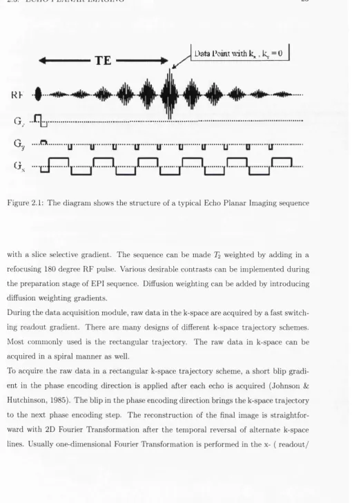
Figure 2.1: The diagram shows the structure of a typical Echo Planar Imaging sequence

with a slice selective gradient. The sequence can be made T2 weighted by adding in a

refocusing 180 degree RF pulse. Various desirable contrasts can be implemented during the preparation stage of EPI sequence. Diffusion weighting can be added by introducing diffusion weighting gradients.

During the data acquisition module, raw data in the k-space are acquired by a fast switch ing readout gradient. There are many designs of different k-space trajectory schemes. Most commonly used is the rectangular trajectory. The raw data in k-space can be acquired in a spiral manner as well.

(26)

frequency encoding ) direction. The data needs to be phase corrected before the second Fourier Transformation. This can be done by using the phase information extracted from the navigator echoes, a separate set of echoes acquired without phase encoding (Ordidge

et ai, 1994; Kelley & Ordidge, 1993; Bruder et ai, 1992). In the project, all the EPI data was phase corrected using a MATLAB program developed by the author.

Any hardware imperfection and magnetic field inhomogeneity introduce additional time shift and phase evolution in the raw data. Because in EPI, alternate k-space lines are acquired with gradients of opposite polarities, the raw data need to be temporally reversed, which shifts this additional evolution in time and phase towards opposite direc tions between two neighbouring k-space lines. Without correction, this shift will lead to formation of a ghost at a position shifted by half of the FOV, after image reconstruction. The correction is usually done by using the phase information extracted from a set of navigator echoes. Each navigator echo is a representation of the projection of all the spins contained in a plane perpendicular to the direction of frequency encoding. Either the same number of navigator echoes as the number of lines in the image is acquired, or only a few navigator echoes are used. It has been shown that using two navigator echoes to perform the phase correction is more effective in reducing the N/2 ghost than using the same number of echoes as the number of lines in the image (Wong, 1992). In the work described in Chapter 4, three navigator echoes were acquired instead of two, to compensate for the fact that the echoes were acquired at different echo times with different off-resonance effect (Heid, 2000).

Throughout the project, the navigator echoes were acquired immediately before the EPI readout began along the frequency encoding direction, with the phase encoding gradient switched off. After the acquisition of the navigator echoes, the phase difference between the alternate lines was extracted at each point, and was subsequently applied to phase correct the original data. The final image is produced after a second Fourier Transfor mation performed in the y- ( phase encoding ) direction.

(27)

2.3. ECHO PLA N AR IMAGING 25

The k-space trajectory will be in a zigzag format. The k-space trajectory may be re- gridded to a rectangular format before the image reconstruction.

The EPI sequence is demanding because the system needs to be able to provide stable switching gradients of opposite polarities within a very short time. The advantage of EPI is that it provides an ultra-short acquisition time. The SNR per unit time is relatively high compared with conventional imaging technique. Yet, the image quality tends to be inferior due to the relatively long signal acquisition time.

In addition to the single shot technique, the raw data in EPI sequences can be acquired within several excitations (Chapman et n/., 1987; Rzedzian, 1987). Each excitation only acquires part of the data in k-space. The raw data are spliced together later prior to image reconstruction. The details of the multiple shots techniques will be discussed in Section 4.1.

2.3.3 H ardw are D em and

A major hardware design consideration in EPI is the requirement of regularly producing large, stable and fast switching gradients. Most modern clinical scanners can provide reasonably reliable and stable systems for EPI acquisition. Thus, in this section we are only discussing the requirements instead of presenting a practical solution. An under standing of the requirement may help the EPI sequence developer to identify the source of ghosts and artefacts.

The rigorous demand on the system hardware arises from the fact that the data are acquired from a train of echoes by one single RF excitation before the signal is destroyed by the T2/ T2 relaxation. The whole acquisition time for one slice of image in the human

(28)

2.3. ECHO P LAN AR IMAGING 26

rably shorter than in any other conventional MR imaging sequences (Bowtell Sz Schmitt, 1998).

The spatial resolution of the image, FOV/N , is inversely proportional to the gradient strength G and the acquisition time for one echo r as in Equation 2.4.

^ =

9

% ;

(

2

.

4

)

As the acquisition time r decreases, to maintain the same spatial resolution, the gradient strength G has to increase. However, in EPI the echoes are acquired by a fast switching gradient. If the spatial resolution is not to be compromised, it is necessary to reverse a large gradient very quickly. The large fast switching gradient system requires a highly efficient gradient coil of low inductance, and a powerful amplifier. This normally requires specially designed switching circuitry such as an EPI booster circuit. The design of an EPI booster circuit is crucial to the performance of EPI sequences in the scanner. The time between each sampling point in the readout direction is which is less than 15 //sec in the above example. The analogue-to-digital converter needs to be very effi cient. Current performance in most state of the art scanners is about 16 bit complex data sampling at a rate of 1 MHz.

(29)

2.4. DIFFUSION WEIGHTED M RI 27

2.4 Diffusion W eighted M RI

Diffusion is the result of Brownian motion, which arises from the random thermal agita tion for all particles at above absolute zero temperature. It has been of growing interest in the measurement of diffusion in vivo since the late 1980s. Diffusion weighted MR images provide important information in the early diagnosis of acute stroke and other neurological disorders. The availability of Echo Planar Imaging sequences to clinical MR scanners makes diffusion weighting imaging possible with satisfactory diffusion contrast and whole brain coverage within a few tens of seconds.

In the following section, the history and theory of DWI will be presented.

2.4.1 H istory o f Diffusion W eighted M R I

Although early studies in the effect of diffusion on NMR by Hahn (Hahn, 1950) and Carr-Purcell (Carr &: Purcell, 1954) etc suggest that NMR can be used to measure the value of self diffusion, it is the work of Stejskal and Tanner in 1965 (Stejskal Sz Tanner, 1965) that forms the foundation of most of the diffusion studies in MRI at this time. The experiment consists of a Spin Echo sequence with a pair of long duration gradients on both sides of the 180-degree RF pulse. The gradient amplitudes and durations are carefully calculated so th at the dephasing from one gradient is completely rephased by the other after the 180 degree RF pulse for the static spins. Diffusion causes incomplete rephasing and a reduction in the net signal. The diffusion coefficient is then derived with Equation 2.1 2, which will be described in detail later.

(30)

2A. DIFFUSION WEIGHTED M RI 28

The applications of diffusion weighted MRI are mainly focused on two fields: stroke and fiber tracking, as described in Chapter 1. In 1990 Moseley et al demonstrated that a re duction of apparent diffusion coefficient can occur within 5 minutes of the onset of acute stroke, which is much earlier than changes in conventional T\ or Tg weighted images (Moseley et al, 1990b). Combined with perfusion weighted MRI, the diffusion weighted image provides important information about diagnosis and therapy planning of stroke patients (Sorensen Sz Buonanno, 1996).

Further applications of diffusion weighted MRI result from the observation that the dif fusion in human brain is mainly anisotropic in certain tissues (Pierpaoli & Basser, 1996). New techniques such as Diffusion Tensor Imaging (DTI) evolved from isotropic Diffu sion Weighted MRI, which provides full characterisation of diffusion in all directions in biological environments (Basser et al, 1994a). Because the diffusion in white matter in the brain mainly follows the direction of fiber tracts, it is potentially possible to map the direction of neuronal fibers with the information contained in the eigenmatrix of the measured diffusion tensor. The result from neuron fiber tracking offers important insight into the understanding of brain connectivity.

2.4.2 P ick’s Laws o f Diffusion

Pick’s first law of diffusion states that the flux J of diffusing particles at position r in time

t is proportional to the concentration gradient of the particles, VC. The proportionality constant D is the diffusion coefficient or diffusivity.

J{r,t) = - D - V C { r , t ) (2.5)

(31)

2.6:

I (2 6)

This leads to Fick’s second law of diffusion as in Equation 2.7:

= - V J ( r , t) = V ( D ■ V C(r, t)) = D ■ V"C(r, t) (2.7)

To measure the diffusion coefficient, conventionally the concentration profile is monitored over a period of time using radioactive or fluorescent-labeled tracers. Such techniques have been applied successfully in biological tissues but because of their intrinsic inva siveness, they cannot be used in humans in vivo.

2.4.3 E instein E quation

If the density of the particles at position ro is p(ro), the probability of finding the particle at position r moving from the original position ro after an observation time t is P (r, ro, t).

The probability density can be expressed in Equation 2 . 8

P (r, t) = j p{ro) • P(ro, r, t)dro (2.8)

Fick’s second law of Diffusion can be deduced for the probability density, as in Equation 2.9

— =Z) - V^P( r o, r , t ) (2.9)

(32)

P(ro, r,t) = { / ^ ) -e (2.10)

y'(47T ■£)•*)

The solution to Equation 2.10 leads to the Einstein Equation of Diffusion (Einstein, 1926) as in Equation 2.11

< { r - r o Ÿ > = 6 - D - t (2,11)

The Einstein Equation of diffusion states that the mean square distance of movement of a particle from position ro to position r depends on the time of observation t. The diffusivity can be directly inferred from Einstein Equation by measuring the second mo ment of the conditional probability distribution of the diffusing particles. This approach is amenable to measurements using NMR and MRI.

2.4.4 M easuring D iffusion w ith M R I

The effect of water diffusion on the MR signal is mainly signal attenuation from spin dephasing. The signal attenuation is the result of gradient activity and diffusion.

The conventional way of measuring diffusion coefficient with MRI is using a simple pair of bipolar gradients in a Gradient Recalled Echo sequence or a pair of unipolar gradi ents on both sides of the refocusing 180-degree RF pulse in a typical Spin Echo type sequence. Figure 2 . 2 shows the structure of such a Spin Echo type diffusion weighted

EPI sequence. The applied gradient will lead to additional spin dephasing and thus signal decay. If there is no diffusion in the medium, this additional signal dephasing will be refocused by the second gradient. The signal acquired during the readout period will only experience the spin-spin relaxation.

(33)

2.4. DIFFUSION WEIGHTED MRI 31

EPI Acq.

►

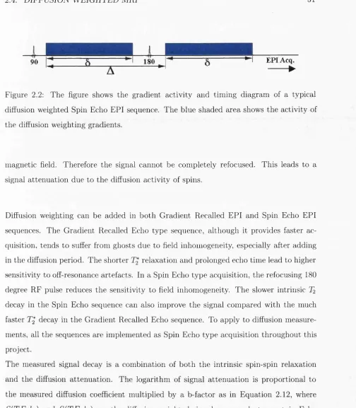
Figure 2.2: The figure shows the gradient activity and timing diagram of a typical diffusion weighted Spin Echo EPI sequence. The blue shaded area shows the activity of the diffusion weighting gradients.

magnetic field. Therefore the signal cannot be completely refocused. This leads to a signal attenuation due to the diffusion activity of spins.

Diffusion weighting can be added in both Gradient Recalled EPI and Spin Echo EPI sequences. The Gradient Recalled Echo type sequence, although it provides faster ac quisition, tends to suffer from ghosts due to field inhomogeneity, especially after adding in the diffusion period. The shorter relaxation and prolonged echo time lead to higher sensitivity to off-resonance artefacts. In a Spin Echo type acquisition, the refocusing 180 degree RF pulse reduces the sensitivity to field inhomogeneity. The slower intrinsic T2

decay in the Spin Echo sequence can also improve the signal compared with the much faster 7^ decay in the Gradient Recalled Echo sequence. To apply to diffusion measure ments, all the sequences are implemented as Spin Echo type acquisition throughout this project.

The measured signal decay is a combination of both the intrinsic spin-spin relaxation and the diffusion attenuation. The logarithm of signal attenuation is proportional to the measured diffusion coefficient multiplied by a b-factor as in Equation 2.12, where

S{TE^bi) and S{TE^b2) are the diffusion weighted signal measured at a certain Echo

Time (TE) with different b-factors 61 and 6 2.

(34)

The b-factor is a constant which describes the sensitivity of the MR sequence to diffusion effects, including the strength, duration and the time separation of the diffusion weighting gradients. It is defined in the Equations 2.13 and 2.14

r T E

b= (2.13)

Jo

fc(t) = 7 - (2.14)

Jo

where G{t') is the effective gradient. In a Gradient Recalled Echo type experiment, the effective gradient in this equation has the same sign as the real gradient. In a Spin Echo type experiment, the sign of the effective gradient should be reversed after each 180 degree RF pulse.

If the ramp of the gradient can be ignored, the b-factor in a typical Spin Echo sequence, such as in Figure 2.2, can be calculated by a simple formula as in Equation 2.15

6 = 7^ ■ • 5^ • (A - ^) (2.15)

where G is the gradient strength and 7 is the gyromagnetic ratio.

To measure the diffusion coefficient as in Equation 2.1 2, normally two images are ac

(35)

2.4.5 C hoosing th e b-factor

The choice of b-factor depends on several factors. During DTI sequence development, usually an optimised or desired b-factor is chosen. Because the b-factor of the sequence depends on the gradient strength and diffusion mixing time, the sequence is normally designed using the shortest echo time according to the maximum gradient that is avail able.

To increase the diffusion weighting, a larger b-factor is required. W ith the same gradient system available, the diffusion time has to increase, as was given in Equation 2.15. The final image will suffer longer T2 relaxation and stronger diffusion attenuation and thus, be

of much smaller SNR. The accuracy of diffusion measurement will be affected. It is thus essential to choose an optimised b-factor which provides appropriate diffusion weighting and maintains the best SNR in the images. Xing et al calculated the optimised b-factor according to the SNR in the diffusion weighted images (Xing et al., 1997). Other optimal data collection schemes have been devised for isotropic media, or for the estimation of the ADC along one direction (Ahn et al., 1986; Prasad & Nalcioglu, 1991). Armitage et al designed an optimised scheme based on the SNR in the calculated diffusion tensor trace map (Armitage & Bast in, 2001). All these works assumed a particular b-factor can be achieved within a short echo time. In the following section the relationship between the echo time and the b-factor will be taken into consideration in the optimization of the b-factor.

In MRI, the signal in the image depends on the T2 relaxation and diffusion attenuation.

It is difficult to estimate the original signal So, and the T2 in the brain can vary over

(36)

The error in the estimation of ADC, 6D, is from the error in the measurements of

S( TE ,bi ) and S ( T E , b2) as in Equation 2.17.

SD =

This leads to

ÔD

SS{TE) (6i - 6 2) \

1 2 1 2 . gfca-D I

---(_______ ) + ( ) = —--- : --- + e2.(6i -62)D

^S(TE,bi)^ ^'^S(TE,b2)^ ( b i - b 2 ) ‘ So ^

(2.18)

If we assumed th at 62 « 0 and b = bi, we have to minimise the following expression:

TE ( b )

e ^2

N = ■ v T + e ^ (2.19)

The echo time TE depends on the b-factor chosen. In a Spin Echo experiment as in Figure 2.2, it is reasonable to assume that both A and 5 are approximately equal to

TE/2. The b-factor can thus be expressed as a function of echo time TE as

b = k ‘TE^ (2.20)

where A: = ^ • 7^ •

Thus, we have

and

TE{b) = {^) (2.21)

(37)

2.5. DIFFUSION TENSOR IMAGING 35

f . O (2.23)

( - )

Figure 2.3 plots the value of N against b-factor for 10 different diffusion coefficients over a range of T2 in the brain.

In our experiment, the maximum effective gradient used in the tetrahedral diffusion en coding scheme (Papadakis et al, 1999) is Gmax = 16 - y/2mT/m. If we assumed that the ADC is approximately 0.9 • 10“^m^/sec and T2 is about 100 msec in human brain, the

optimised b-factor is approximately 998 • 10^sec/ c a l c u l a t e d from the figure.

In the following experiments, two sets of b-factors were used. The b-factors chosen were 992.88 • 10^sec/m? in the high diffusion weighted sequences and 96.96 • 10®sec/m^ in the low diffusion weighted sequence. This will lead to a difference of the b-factors of 895.92 • 10®5ec/m^, which is quite close to the optimised value. The b-factor used in the selective averaging experiment is slightly lower at 868- 10®sec/m^ which will be described in more details in Chapter 4.

2.5 D iffusion Tensor Im aging

(38)

2.5. DIFFUSION TENSOR IMAGING 36

0 = 1 . 2 * 1 0 - 9 m 2 /s e c 0 = 1 . 2 * 1 0 - 9 m 2 /* # o

0.5

0 = 0 . 3 * 1 0 - 9 m 2 /6 e c 0 = 0 . 3 * 1 0 - 9 m 2 /s « o

b-factor

,1 0'

b-factor

2.S 2.»

0 = 1 .2 * 1 0 - 9 m 2/*ec

0 = 1 .2 * 1 0 - 9 m 2 /se c

0.5 0.5

0 = 0 .3 * 1 0 - 9 m 2 /s« c _{0 = 0 .3 * 1 0 - 9 m 2/**o}

SMI tN4

t*M

I2M IMI UN l#W tan

b-factor

Figure 2.3: The figure plots the value of N against b-factor for 10 different diffusion coefficients ranging from 0.3 • 10“^m^/sec to 1.2 • 10~^m^/sec with increment of 0.1 • 10“®m^/sec for a range of Tg. The b-factor is given in unit of 10®sec/m^.

Top Left: T2 = 70 msec

(39)

2.5.1 D iffusion A nisotropy in H um an E nvironm ent

The measurement of the diffusion coefficient from the Einstein Equation 2.11 assumes th at the diflPusing particles are in free motion. However, in biological tissues one cannot assume a homogeneously free environment. The diffusing particles within and between the cells are bound to hit obstacles, organelles and cell membranes etc. Considering a typical cell of size 10 fim in diameter, it takes less than 4 msec for the water molecule to reach the boundary from the centre of the cell, according to predictions from the Einstein Equation. However, the measured diffusion coefficient in the human brain is approximately 10“® • m^/sec, while the value measured in free water is considerably larger at approximately 3.5 • 10“®m^/sec. This suggests th at hindrance to the mobility of molecules occurs within and between the cells. Thus the diffusion is no longer free and isotropic in the biological environment (Turner, 1998).

(40)

2.5.2 In troduction to th e D iffusion Tensor

The diffusion tensor consists of a 3 by 3 matrix which characterises the diffusion in all the directions as in Equation 2.25 (Basser et al, 1994a; Basser et al, 1994b; Basser & Pierpaoli, 1996).

D = (

\

Dxy A

Dyx _^yy A

Dzx Dzy D, yz

\

{2.2b)

The diffusion coefficient is positive definite. The measured diffusion coefficient in the xy direction is the same as the one in the yx direction and likewise for the diffusion coefficients measured in all the other off-diagonal directions. The components of the diffusion tensor in the diagonal directions define the diffusion in the three principal directions while the off-diagonal components describe the effect of correlation among the perpendicular diffusion weighting directions.

Fick’s law of diffusion can be extended to the diffusion tensor form as in the following Equations 2.26 and 2.27:

And

^ J^{x,y ,z,t) ^ Jy{x,y,z,t)

y J^{x,y,z,t) j

^ dc{x,y,z,t) \ ( dt

dc{x,y,z,t) dt dc(x,y,z,t)

dt

D x x D x y D x z O y x ^ y y D y z D z x D z y D z z

\

X

^ dc(x,y,z,t) ^ dx dc{x,y,z,t) dc(x,y,z,t)

dz

D x x D x y D x z D y x D y y D y z D z x D z y D z z

X V

^ c(x, y, z, t) ^ c{x,y ,z, t)

y c {x, y, z,t ) j

(2.26)

(2.27)

2.5.3 D efinition o f b-m atrix

(41)

the coordinate systems of the eigenmatrix of the tensor and the scanner. This requires at least six measurements with various non-linear diffusion encoding directions and one ad ditional measurement without diffusion weighting to obtain the value S { T E , blow) (Basser & Pierpaoli, 1998). With Equation 2.12, diffusion in the biological environment can be expressed as in Equation 2.28

bxx bxy bxz byx b y y byz

bzx ^zy ^zz

X

(

\

Oxx Dxy D:

Dyx Dyy D,

Dzx Dzy D.

yz

\

/

(2.28)

where S { T E , bm) is the signal acquired from the m th measurement and the S { T E , bi^yw)

is the signal with low or non diffusion weighting acquired at the same echo time TE. In the Spin Echo experiment as described in the previous example in Figure 2.2, the elements bijjori,j=x,y,z in the b-matrix of Equation 2.28 can be calculated from Equation 2.29

(2.29) Where Gi and Gj are the diffusion weighting gradients applied in the i and j directions respectively.

2.5.4 D isp lay o f th e D iffusion Tensor

(42)

Eigenm atrix o f th e Diffusion Tensor

The orientation of the intrinsic diffusion in the human environment is generally differ ent from the directions used in the diffusion encoding scheme during the measurements. The diffusion tensor is diagonal in a coordinate system the axes of which are given by the eigenvectors of the tensor matrix D, After acquiring the full diffusion tensor, it is necessary to rotate the tensor matrix to its eigenmatrix. The directions of the three eigenvectors Ai, A2, A3 point to the real directions of the principal diffusions and the

corresponding eigenvalues 6 1,6 2 ,6 3 show the diffusion in the respective direction. The

eigenvalues thus can reflect the true diffusion in different directions within the voxel of interest.

The eigenvalues are often sorted according to the absolute values. In an ideally isotropic environment such as free water, the three eigenvalues should be the same. Yet, in bi ological tissues, the absolute values of the sorted eigenvalues can vary within a wide range and the largest eigenvalues can be up to ten times the smallest eigenvalues. Thus eigenvalues of the diffusion tensor matrix provide a good way to measure the diffusion anisotropy in the biological environment.

The Diffusion Tensor as Ellipsoids

One of the most straightforward ways of displaying the diffusion tensor is to depict it as an ellipsoid on a voxel by voxel basis as shown in Figure 2.4 (Basser et al, 1994b; Basser

et ai, 1995).

(43)

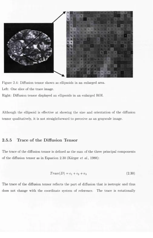
Figure 2.4: Diffusion tensor shown as ellipsoids in an enlarged area. Left: One slice of the trace image.

Right: Diffusion tensor displayed an ellipsoids in an enlarged ROI.

Although the ellipsoid is effective at showing the size and orientation of the diffusion tensor qualitatively, it is not straightforward to perceive as an grayscale image.

2.5.5 Trace of the Diffusion Tensor

The trace of the diffusion tensor is defined as the sum of the three principal components of the diffusion tensor as in Equation 2.30 (Karger et «/., 1988):

Trace{D) = ei F € 2 F (2.30)

(44)

invariant and provides an estimation of the bulk diffusion.

Interestingly, though the ADCs measured in white matter, gray m atter and CSF in human brain are different, the image of trace looks relatively uniform. Typical trace values measured in the brain (Shimony et ai, 1999) are around 2.17*10“^m^/sec in ROIs in Splenium of Corpus Callosum and 2.16-10“®m^/sec in Genu of Internal Capsule in white matter. In gray matter it is around 2 . 3 9 - / sec in ROIs in the head of Caudate Nucleus and 2.65-10“^m^/sec in Frontal CM.

Throughout the project, the trace is presented as the mean value of the bulk diffusion, trace/3, which reflects the isotropic component of the diffusion.

Figure 2.5 shows the trace and three sorted eigen images from the same slice in the human brain displayed on the same windowed scale.

2.5.6 C haracterising D iffusion A n isotrop y

There have been several different ways to characterise diffusion anisotropy in the human brain. Some definitions of diffusion anisotropy are rotationally variant, and are thus susceptible to the changes in the diffusion encoding scheme. Others are rotationally invariant, and remains constant regardless of the orientation of the coordinate system of reference used for diffusion weighting gradients.

The ratios of the eigenvalues reflect the extent of diffusion anisotropy. They are the most intuitive and simplest way to characterise the diffusion anisotropy as defined in Equation 2.31(Douek et o/., 1991) and 2.32 (Pierpaoli & Basser, 1996).

volume ratioi = — (2.31)

^3

volume ratio2 = (2.32)

€2 + 63

(45)

eigen-2.5. DIFFUSION TENSOR IMAGING 43

I

%

*r

f à

^ ^ *

•* f' I K «#"' m''«

■ ■■ - y V . •

Figure 2.5: The figure shows the trace image and three sorted eigenimages of the same slice. Images are acquired with the same parameters used in the in vivo experiment in Chapter 3: using a single shot EPI sequence, matrix size of 64 by 64, isotropic voxel size of 3 mm, standard diffusion encoding as described in Section 2.4. Images are displayed at the same windowing scale.

Top Left: Image of the trace/3 from one slice of the brain. Top Right: Image of the largest eigenvalue from the same slice.

(46)

values, and are thus particularly susceptible to the low SNR of the diffusion weighted images (Mehta, 1991; Ahrens et ai, 1998).

Relative Anisotropy (RA) and Fractional Anisotropy (FA) are both rotationally invari ant and independent of the order of the eigenvalues, which avoids the sorting errors as encountered in Equation 2.31 and 2.32 (Basser & Pierpaoli, 1996).

Relative Anisotropy is the ratio of the anisotropic component divided by the isotropic component of the diffusion tensor as in Equation 2.33. Similarly, Fractional Anisotropy is defined in Equation 2.34.

pA _ (^1 - + (^2 - «3)^ + (€ 3 - ,

- (e, + c. + .3)

F A = - f s)' + - fs )' + (^3 - f i) : (2.34)

yj2 • (ei^ 4- + 63^)

(47)

Figure 2.6: The figure shows one slice of brain images of the Relative Anisotropy map and Fractional Anisotropy map. Parameters used are the same as in Figure 2.5.

(48)

2.6. PROTOCOLS IN MEASURING THE DIFFUSION TENSOR 46

2.6 P rotocols in M easuring th e D iffusion Tensor

In this project, all the experiments were carried out in a 2 Tesla MRI whole body scanner ( Siemens Magnetom Vision, Erlangen Germany ) in a passively shielded magnet. The maximum gradient strength available is 25 m T /m .

The water phantom used in the experiments is a standard phantom made by Siemens Erlangen. It is made of 2.571 liter of water in a spherical container doped with 1.25 g

N i S 0 4 • diJsO.

A gel phantom was made and used in the experiments as well. It was stored in a spherical container and doped with 6.65 % Acrylamide, 0.35 % Bisacrylamide, 0.1 % Ammonium Persulphate and 0.076 % TEMED. The recipe was proposed by Dr. Denis LeBihan from Commissariat a l’Energie Atomique, Orsay, France, through private communication. The processing of the raw data, including the extraction of phase information from the navigator echoes, correction of the phase evolution in the raw data, the image reconstruc tion and the calculation of the diffusion tensor images and the Fractional Anisotropy maps was all implemented by the author and performed with MATLAB (The Math- works, Natick, Mass., USA).

When it is necessary to select a Region Of Interest ( ROI ), it was drawn by hand along the boundary of the structure of interest or in a region as large as possible yet without inclusion of overlapping ghosts. The size of the ROI thus varied. In a multiple measure ment, the first measurement was used if not specified in the text.

None of the data from separate scans were co-registered except those particularly speci fied. This is to avoid rotation of the diffusion tensor.

(49)

Order of measurements Read Out Phase Encoding Slice Selection

1 G 0 0

2 0 G 0

3 0 0 G

4 _v/2G a 0

5 a 0 _x/2a

6 0 _^/2a _v/2a

Table 2.1: The table shows the strength and directions of the diffusion weighting gra dients in the standard diffusion encoding scheme from six high diflPusion weighted mea surements. G is the strength of the diffusion weighting gradient.

directions and three off-orthogonal axes along the combined direction of the phase en coding/ slice selection, phase encoding/ read out and slice selection/ read out directions.

In the second scheme, the diffusion weighting gradients are applied to the tetrahedral directions as in Table 2.2 and was referred to as the tetrahedral diffusion encoding scheme throughout the project (Papadakis et o/., 1999).

(50)

Order of measurements Read Out Phase Encoding Slice Selection

1 -G G 0

2 -G 0 G

3 G G 0

4 G 0 G

5 0 -G G

6 0 G G

(51)

C hapter 3

Single Shot D iffusion Tensor E P I

To demonstrate the stability and reproducibility of the diffusion tensor imaging, stan dard single shot EPI was used as the template. Diffusion weighting gradients were added in 6 directions using the standard diffusion encoding scheme as described in. Section 2.6 in Chapter 2. The acquisition time per echo was 1024 fis, and the matrix size was 64 by 64. The field of view was 192 mm by 192 mm and the slice thickness was 3 mm, resulting in an isotropic voxel size of 3 mm. The sequence was tested in vitro on a water phantom and in vivo on six healthy volunteers which was repeated twice.

For high diffusion weighted measurements, 15 averages of each measurement were ob tained. For low diffusion weighted measurements, 12 averages were measured. The effective echo time was 102 msec and the k-space was sampled asymmetrically by acquir ing the central k-space line after 25 % of the EPI echo train acquisition, thus reducing the echo time (Hennel & Nedelec, 1995).

The b factors chosen were 923 -10®sec/m^ for measurements in the 3 principal directions, and 461 TO^sec/m^ for measurements along the off-diagonal directions. The b-factor for the low diffusion weighting measurement was 117 -lOPsec/mP.

(52)

3.1. PHANTOM STU D Y 50

3.1 P hantom Study

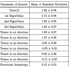
In the phantom study, a Siemens phantom made from doped water was used in all the experiments. The values of the trace/3, eigenvalues, Fractional Anisotropy of the tensor from a region of interest are shown in Table 3.1. The diffusion coefficient measured at 1 ATM and 20 Celsius degree was 1.95'10“®m^/sec, which is close to the value of 2.05 '10~^m^/sec for pure water reported by Harris et al (Harris & Woolf, 1980) under similar conditions. The measured Fractional Anisotropy of 0.12 shows reasonable low directionality in free water, which is comparable to the simulated data from Pierpaoli et al for isotropic material (Pierpaoli & Basser, 1996).

Figure 3.1 and Figure 3.2 show the calculated tensor images of the phantom. Both the trace image and the images of eigenvalues are relatively ghost free. All the images of the eigenvalues are quite similar, which suggests low anisotropy, as expected. Fractional Anisotropy maps show that the phantom has low diffusion anisotropy inside the phantom with a bright ring at the edge, which could be due to vibration of the scanner bed during the data acquisition, residual eddy current or a susceptibility artefact.

3.2 Study on H ealthy Volunteers

To study the reproducibility of the sequences on humans, 6 healthy volunteers, including four male and two female (aged 33.5 ± 5.54 years old, between 26 to 40) were scanned twice with the same protocol. After data processing, 8 parameters are presented here for comparisons: Fractional Anisotropy, trace/3, three sorted eigenvalues and three apparent diffusion coefficients along the main axes.

(53)

3.2. STU D Y ON HEALTH Y VOLUNTEERS 51

Parameter of Interest Mean ± Standard Deviation Trace/3 1.95 ± 0.08

1st Eigenvalue 2.15 ± 0.08 2nd Eigenvalue 1.89 di 0.06 3rd Eigenvalue 1.80 ± 0.07 Tensor in xx direction 1.89 ± 0.07 Tensor in yy direction 1.87 ± 0.06 Tensor in zz direction 2.08 ± 0.06 Tensor in xy direction -0.03 ± 0.05 Tensor in xz direction 0.06 ± 0.06 Tensor in yz direction -0.11 ± 0.03 Fractional Anisotropy 0.12 ± 0.03

(54)

3.2. STUDY ON HEALTHY VOLUNTEERS 52

Figure 3.1: The figure shows the trace and eigenimages acquired by the single shot EPI sequences.

(55)

3.2. STUDY ON HEALTHY VOLUNTEERS 53

/ ••• / V

^ __ “v

(56)

the ROIs.

The mean values of Fractional Anisotropy in white m atter 0.92, and in gray m atter 0.31, are higher than the values reported by other groups ( 0.73 in Splenium Corpus Callosum and 0.20 in the head of Caudate Nucleus) (Shimony et al., 1999). The variation among the six subjects in the calculated Fractional Anisotropy is larger in gray matter ( 19.8 % for the first measurement and 18.1 % for the second measurement ) and CSF ( 28.9 % and 16.2 % respectively ) than white matter ( 3.8% and 3.7 % respectively ). The variation in the trace is similar among different ROIs in the six subjects, which is approximately

10 %.

The relative deviation A between two measurements is calculated for the Fractional Anisotropy, trace/3 and the first eigenvalue for all the six subjects. It was calcu lated as the squared root of the square of the differences divided by the mean values: A = TaWe 3 . 3 shows the A in % in three ROIs described

above.

The variation between the measurements in various tissue types of the brain shows sat isfactory reproducibility in the case of the single shot DT-EPI sequences. The variation among the subjects and between measurements can be affected by several factors such as the variations in the choice of ROIs, tissue type, the SNR in the original diffusion weighted images and the intrinsic reproducibility of the sequence. In Table 3.3, there is no clear difference between the results in different ROIs. The parameters in CSF should be close to that of pure water. The variation between measurements in CSF is probably caused by motion artefact associated with pulsatile inflow. Here CSF in general shows greatest variations in these parameters between measurements.

(57)

Parameters Posterior Corpus Callosum Pericalcarine 1st session 2nd session 1st session 2nd session 1st Eigenvalue 1.39 di 0.17 1.40 ± 0.12 1.20 ± 0.12 1.16 ± 0.08 2nd Eigenvalue 0.42 ± 0.08 0.42 ± 0.07 0.96 d: 0.11 0.93 ± 0.08 3rd Eigenvalue 0.04 ± 0.09 0.04 ± 0.09 0.75 ± 0.10 0.75 ± 0.10 Tensor in xx direction 0.92 ± 0.16 0.94 ± 0.13 0.97 ± 0.09 0.92 ± 0.09 Tensor in yy direction 0.43 ± 0.12 0.46 di 0.10 0.95 ± 0.12 0.92 ± 0.07 Tensor in zz direction 0.50 ± 0.04 0.46 di 0.04 1.00 ± 0.11 0.99 ± 0.09 Trace/3 0.63 ± 0.07 0.63 di 0.07 0.97 ± 0.10 0.94 ± 0.08 Fractional Anisotropy 0.91 ± 0.03 0.92 di 0.03 0.31 ± 0.06 0.31 ± 0.05

CSF

1st session 2nd session 1st Eigenvalue 3.39 ± 0.38 3.39 ± 0.44 2nd Eigenvalue 2.82 ± 0.35 2.79 ± 0.50 3rd Eigenvalue 2.28 ± 0.40 2.27 ± 0.40 Tensor in xx direction 2.74 ± 0.36 2.69 ± 0.53 Tensor in yy direction 2.91 ± 0.48 2.80 ± 0.35 Tensor in zz direction 2.85 ± 0.37 2.96 ± 0.50 Trace/3 2.83 ± 0.36 2.82 di 0.44 Fractional Anisotropy 0.26 ± 0.08 0.26 ± 0.04

(58)

3.2. STU D Y ON H EALTH Y VOLUNTEERS 56

Trace

3 5

CSF

2.5

1.5

Gray Matter

0.5

White Matter

6 Subject

Trace

3.5

CSF

2.5

1 . 6

Gray Matter

0.5

W hite Matter

eSubject

Figure 3.3: The figure shows the calculated trace/3 between two measurements among the six healthy subjects in different ROIs. The values are given in units of / sec.

(59)

1.4

1.2

0.8

0.6

Gray Matter

0.4

0.2

tS F

6 Subject

1.4

FA