Performance Analysis of Compressive Sensing Algorithms
for Image Processing
Sonia Gandhi1, Deepti Khanduja2 and Neelu Pareek3
1 Department of Electronics and Communication, Vivekananda Global University, Jaipur, Rajasthan, India
2
Department of Computer Science, Swami Keshwanand Institute of Technology, Jaipur, Rajasthan, India
3 Department of Electronics and Communication, Vivekananda Institute of Technology, Jaipur, Rajasthan, India
Abstract
Compressive sensing is an emerging research field that has applications in signal processing, error correction, medical imaging, seismology, and many more other areas. Compressive sensing has a wide range of applications that include error correction, imaging, radar and many more. We present a new algorithm (the Modified Orthogonal Matching) for signal reconstruction in compressive sensing. We have given a basic frame work for our algorithm. This algorithm is able reconstructs the denoised Image efficiently. In addition we have compared the simulated results of BP with OPM and modified OMP with standard OMP in sense of PSNR and Computational Time. Simulation results show that the modified algorithm outperforms existing compressed sensing reconstruction methods.
Keywords: Orthogonal Matching Pursuit, Basis Pursuit
1. Introduction
Compressive sensing, also referred to as compressed sensing or compressive sampling, is an emerging area in signal processing and information theory which has attracted a lot of attention recently. The motivation behind compressive sensing is to do “sampling” and “compression” at the same time. In conventional wisdom, in order to fully recover a signal, one has to sample the signal at a sampling rate equal to or greater than the Nyquist sampling rate. However, in many applications such as imaging, sensor networks, astronomy, high-speed analog-to-digital compression and biological systems, the signals we are interested in are often “sparse” over a certain basis. For example, an image of a million pixels has a million degrees of freedom, however, a typical interesting image is very sparse or compressible over the wavelet basis. Only a small fraction of wavelet coefficients, say, one lakh out of a million wavelet coefficients, are significant in recovering the original images, while the rest of wavelet coefficients are “thrown away” in many compression algorithms. This process of “sampling at full rate” and
then “throwing away in compression” can prove to be wasteful of sensing and sampling resources, especially in application scenarios where such resources as sensors, energy, and observation time etc. are limited. Instead of thinking in the traditional way, compressive sensing promises to recover the high-dimensional signals exactly or accurately, by using a much smaller
number of non-adaptive linear samplings or
measurements. In general, signals in this context are represented by vectors from linear spaces, many of which in the applications will represent images or other objects. The fundamental theorem of linear algebra, “as many equations as unknowns,” tells us that it is not possible to reconstruct a unique signal from an incomplete set of linear measurements. However, as discussed earlier, many signals such as real-world images or audio signals are often sparse or compressible over some basis, such as smooth signals or signals whose variations are bounded. This opens the room for recovering these signals accurately or even exactly from incomplete linear measurements. However, even though we know that the signal itself is sparse, it is a non-trivial job to recover the signals from the compressed measurements since we do not know the locations of the non-zero or significant components of that vector. One of the cornerstone techniques enabling compressive sensing is then about efficient and effective decoding algorithms to recover
the sparse signals from the “compressed”
measurements.
2. Literature Survey
In 1965, Logan’s dissertation [1] proved a result now known as “Logan’s phenomenon”: if a continuous-time band-limited signal x(t) is corrupted by noise z and the noise has bounded L1 norm and has a very sparse
can perfectly recover the original signal x. This is remarkable, because it is independent of the magnitude of the error.
The work of [2] proved that recovery of a k-sparse vector from just m Fourier measurements was possible if m ≥ (1 − 1/ (2k)) n, using the unconstrained LASSO formulation [2] also note the pessimistic nature of this bound). Even by 1986, the fact that “it is possible to construct a sparse spike train from part of its spectrum using the minimum l1 criterion” was “well-known (and
believed)” [2]. The 1989 article by Donoho and Stark [3] extended Santosa and Symes results by proving a more general new type of uncertainty principle [4]. The classical time- frequency uncertainty principle says that a signal cannot have small support in both time and frequency. The [3] result extended this result by relaxing the restriction that a signal’s support be on intervals. To be concrete, let x be a discrete signal of length n with discrete Fourier transform X. Donoho and Stark prove
‖x‖₀ ‖X‖₀ ≥n (and hence ‖x‖₀+‖X‖₀ ≥2⎷n) (1)
Intuitively, the result says that there are not many discrete signals that are sparse in both time and frequency. Thus, if a signal happens to be sparse in both time and frequency, it has no “neighboring” signals, and for this reason it is easy to recover. The multiplicative inequality is sharp, because if n = d2, then a Dirac comb of spacing
d has ‖x‖₀=‖X‖₀ =d; this example is also sharp for the additive identity (the additive identity follows from the multiplicative one by the arithmetic geometric mean inequality). Another example is when x is a single Fourier element, in which case ‖x‖₀=n and ‖X‖₀=1, so the multiplicative inequality is sharp but the additive inequality is not. It turns out the additive inequality is only sharp in cases such as n =d2; the situation when n is prime is quite different [5].
Stark in [3] also reports numerical experiments suggesting that much stronger results are possible if the sparsity is “scattered” in a random way, so it is clear that the authors had some insight into what was achievable; their official bound on measurements was the same as Santosa and Symes. It is worth mentioning that their numerical experiments went only as large as n = 256, and it is not easy to distinguish O(n), O√n), and O(log n) growth from experiments with just n = {64, 128, 256}.
This theory in the late 1980s built on empirical work from the previous 15 years,
as different scientific communities were using l1
minimization and/or sparsity. The work in [6] in 1973 argues that the geophysics community should consider l1
regularized problems for the sake of robustness to outliers, using the mean and median estimators as examples. They also argue that l1 generates sparsity,
but only to the extent that there is always a vertex solution to a linear program (so sparsity of a solution can be chosen less than m). In addition to sparsity in space, they give 17 examples of using sparsity in first- and second-differences; this was further explored in the highly influential total-variation (TV) minimization paper in 1992 [7]. Similar works in geophysics, such as [8], cite l1 studies going back to 1964. Incremental results
continued in geophysics, exemplified by [9] in 1994 which cites numerous l1 results from the 1980s. Many
of these works proposed special algorithms to avoid recasting the problem as a linear program (LP). In radio astronomy, the CLEAN algorithm , introduced around 1971, exploits sparsity of radio sources and is similar to a matching pursuit algorithm as shown by [10], though it is not equivalent to l1 minimization (indeed,
the first analysis of CLEAN [11] compares it to l2
minimization). Its idea of exploiting sparsity and post-processing has been extremely useful in astronomy “The impact of CLEAN on radio astronomy has been immense. First, there is the accumulated science from
the telescopes that have used CLEAN— GBI,
MERLIN, WSRT, VLA, VLBI, etc. ... Second, by showing what could be achieved with some post processing, CLEAN has encouraged a wave of innovation in synthesis processing that continues to this day.” The article [12] introduces the authors’ algorithms from 1975 to the application of estimating the transfer function of an unknown medium using ultrasound pulses, and exploits sparsity in the number of layers in most mediums. The algorithm they propose is similar to alternating projections between the time domain (which is sparse) and the frequency domain (where it is assumed that reliable data exists in some band). The 1982 article [13] discusses an application of l1
3. Proposed Algorithm
3.1 Basic Pursuit
The intuitive approach to the compressive sensing problem of recovering a sparse vector x
∈
RN from its measurement vector y = Φx∈
Rm, where m < N, consists in the l0 -minimization problemminx∈ Rn ‖x‖₀ subjected to Φx = y
This is a non convex problem that it is NP-hard in general. However, keeping in mind that ‖z‖qq approach ‖z‖₀
as q>0 tends to zero we can approximate by the problem
minx∈ Rn ‖x‖q subjected to Φx = y (2)
For q > 1, even 1-sparse vectors are not solutions of (2). For 0 < q < 1, (2) is again a no convex problem, which is also NP-hard in general. But for the critical value q = 1, it becomes the following convex problem (interpreted as the convex relaxation of (1).
min Minx𝟄𝟄 Rⁿ ‖x‖₁ subject to Φx= y (3)
This principle is usually called l1 -minimization or basis pursuit.
Basic Pursuit:
Input: measurement matrix Φ, measurement vector y.
Instruction:
x’=arg min ‖z‖1 subject to Φz = y
Output: the vector x’
3.2 Orthogonal Matching Pursuit
Orthogonal Matching Pursuit (OMP) is a greedy algorithm which can reliably recover a signal with nonzero entries in dimension d, given O(m ln d) random linear measurements of that signal. This is a massive improvement over previous results, which
require O(m2) measurements. The new results for OMP are comparable with recent results for another approach called Basis Pursuit (BP). In some settings, the OMP algorithm is faster and easier to implement,
so it is an attractive alternative to BP for signal recovery problems.
3.2.1 OMP for Signal Recovery
This section describes how to apply a fundamental algorithm from sparse approximation to the signal recovery problem. Suppose that x is an
arbitrary s-sparse signal in RN, and let {x1… xN} be a family of measurement vectors. Form an N X d matrix Φ whose rows are the measurement vectors, and observe that the N measurements of the signal can be collected in an N-dimensional data vector y = Φx . We refer Φ to as the measurement matrix and denote its columns by φ1……. Φd.
As we mentioned, it is natural to think of signal recovery as a problem dual to sparse approximation. Since x has only s nonzero components, the data vector y = Φx is a linear combination of columns from Φ. In the language of sparse approximation, we say that y has an s -term representation over the dictionary Φ.
Therefore, sparse approximation algorithms can be used for recovering sparse participate in the measurement vector y. The idea behind the algorithm is to pick columns in a greedy fashion. At each iteration, we choose the column of Φ that is most strongly correlated with the remaining part of y. Then we subtract off its contribution to y and iterate on the residual. One hopes that, after iterations, the algorithm will have identified the correct set of columns.
Algorithm 1 (OMP for Signal Recovery):
INPUT:
•
An N x d measurement matrix Φ•
An N-dimensional data vector y•
The sparsity level s of the ideal signalOUTPUT:
•
An estimate x’ in Rn for the ideal signal•
A set Ʌs containing s elements from {1,….d}•
An N -dimensional residual rm =y – am.PROCEDURE:
1)
Initialize the residual r0 = y, the index set Λ₀ = Ø, and the iteration counter t = 1.2)
Find the index ƛt that solves the easy optimization problemƛt =arg max j=1,….d |(rr-1 𝞿𝞿j)| (4) If the maximum occurs for multiple indices, break the
tie deterministically.
3)
Augment the index set and the matrix of chosen atoms:Ʌt = Ʌt-1U {ƛt} and ɸt =[ɸt-1 𝞿𝞿ƛt ]
We use the convention that is an empty matrix.
4)
Solve a least squares problem to obtain a new signal estimate:mt = arg minx ‖v-ɸt m‖
5)
Calculate the new approximation of the data and the new residualrt = y-at where at = ɸt mt
6)
Increment t, and return to Step 2 if t < m.7)
The estimate x’ for the ideal signal has nonzero indices at the components listed inΛm . The value of the estimate in component Λj equals the jth component of mt.
Steps 4, 5, and 7 have been written to emphasize the conceptual structure of the algorithm; they can be implemented more efficiently. It is important to recognize that the residual is always orthogonal to the columns of Φt. Provided that the residual rt-1 is nonzero; the algorithm selects a new atom at t iteration and the Φt matrix has full column rank. In above case the solution mt to the least squares problem in Step 4 is unique. (It should be noted that the approximation and residual calculated in Step 5 are always uniquely determined.)
The running time of the OMP algorithm is dominated by Step 2, whose total cost is O(mNd). At iteration t, the least squares problem can be solved with marginal cost O(tN).
Despite numerous advantages, OMP is unable to give accurate results in presence of noise. While processing images, it fails to preserve the edges and give blurry result. Thus we modify OMP by using the
property wavelet thresholding which help us to remove noise and get better results. In the modified likewise OMP step by step estimation take place but after predicting the value a threshold will be subtracted thus removing the noise.
3.3 Compressive Sensing in Image Processing
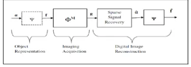
The recently introduced theory of compressed sensing (CS) has attracted the interest of theoreticians and practitioners alike and has initiated a fast emerging research field. CS suggests a new framework for simultaneous sampling and compression of signals. In contrast to the common framework of first collecting as much data as possible and then discarding the redundant data by digital compression techniques, CS seeks to minimize the collection of redundant data in the acquisition step. A natural branch of CS is compressive Imaging (CI). A block diagram for CI with random projections is shown in Fig. 4.1
Fig 1 Imaging scheme of compressed sensing.
The object f consisting of N pixels is
imaged by taking a set, g, of random
projections. One can also think of M as the number of detector pixels. We are taking the case of M <
N, meaning that the captured image is
undersampled in the conventional sense. Ψ is an arbitrary orthonormal signal sparsifying basis (i.e., Fourier, wavelet, or DCT), and g ∈ RM is the acquired image. α ∈ CN is the m- sparse representation of image projected on (Fig. 1), meaning, that the
particular interest here is that it is incoherent for almost all possible choices of the sparsifying operator Ψ. CS theory is that a signal (image) measured with Φ can actually be recovered by l1 -norm minimization, the estimated coefficients vector α is the solution of the convex optimization program
3.4 Modified OMP
In a CS-based image processing system, denoising is very important to improve the quality of images using a reduced amount of data. Especially, it is a challenging problem to remove the noise while preserving image details because of the high- frequency characteristics of the noise. In this CS-based image denoising algorithm, wavelet thresholding is used to remove the effect of noise and efficiently recover the image. Our model contain two steps
(1) Block based compressive sensing and detecting the threshold value for the noisy image.
(2) Reconstruction using modified OMP (OMP with wavelet thresholding).
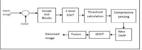
Block-based model sampling for fast CS of natural images, where the original image is divided into small blocks and each block is sampled independently using the same measurement operator. In block CS, the image is divided into small blocks with size of B ×B each and sampled with the same operator. After dividing the images into blocks, wavelet transform is carried out for each block. After transforming the signal in sparse domain, threshold is calculated according to noise level by using Birge and Massart Strategy. After calculating the threshold, the sensing process is done and the modified OMP recover the denoised Image. Figure 3 shows the basic block diagram showing the steps in modified OMP.
Fig 2 Block diagram for CS based image Denoising
3.4.1 Wavelet transform
Wavelet Transform is a mathematical tool used to represent signals (or images) in a domain in which it may be manipulated more effectively. It shares many properties and is similar to the well known Fourier Transform. Both the Fourier and Wavelet Transforms are based on “basis functions”. Unlike the Fourier transform, whose basis functions are sinusoids; Wavelet Transforms are based on small waves, called Wavelets, of varying frequency and limited duration. Wavelet analysis can be used to divide the information of an image into approximation and detail sub signals. The approximation sub signal shows the general trend of pixel values, and three detail sub signals show the vertical, horizontal and diagonal details or changes in the image. If these details are very small then they can be set to zero without significantly changing the image. The value below which details are considered small enough to be set to zero is known as the threshold. The greater the number of zeros the greater the compression that can be achieved.
A. Discrete Wavelet Transform (DWT)
Calculating wavelet coefficients at every possible scale is a fair amount of work, and it generates an awful lot of data. So we choose only a subset of scales and positions based on powers of two, so called dyadic scales and positions, then the analysis will be much more efficient and just as accurate. If the function being expanded is a sequence of numbers, like samples of a continuous function f(x), the resulting coefficients are called the discrete wavelet transform (DWT) of f(x). Figure 3 is a sketch map of one, two and three-level decomposition for two-dimensional wavelet transform DWT.
Fig 3 Schematic diagram of 2D DWT
Fig 4 Multilevel Image Decomposition
B. Haar Wavelet
Any discussion of wavelets begins with Haar wavelet, the first and simplest. Haar wavelet is discontinuous, and resembles a step function as shown in Figure 5
Fig 5 Haar wavelet
3.4.2 Birge and Massart Strategy
Selecting threshold is important for image denoising. A small threshold may yield a result close to the input, but the result may still be noisy. A large threshold on the other hand, produces a signal with a large number of zero coefficients which leads to a smooth signal. Paying too much attention to smoothness, however destroy details in image and may cause blur and artifact.Here we have taken Birge and Massart Strategy for selecting Threshold. This is level wise threshold method which is also provided by Birge and Massart [15]. It uses level-dependent thresholds obtained by the following wavelet coefficients selection rule. Let j be the decomposition level, m be the length of coarsest approximation coefficients over 2 and α>1. The numbers
j, m and j+1define the strategy: at level j +1 (and coarser levels), everything is kept. For level i from 1 to j, the nj larger coefficients in absolute value are kept with:
nj =m ∕ (j+2-i)α
The modified OMP algorithm is given below-
Algorithm 2
Input:
•
Measurement matrix Φ•
Measurement vector Y•
Sparsity level (s)•
Threshold value (t)Output:
• Reconstructed signal x’
• Residual rt= v-at
PROCEDURE:
1. Initialization: residual r₀=v, index data set I= ∅ and iteration t = 1.
1.
Solve optimizationƛt =arg maxj=1,….d | (rr-1 𝞿𝞿j) |
3
. Updateɸt = [ɸt-1 𝞿𝞿ƛt ]
4.
New estimation of signal xt = arg minx ‖v- ɸt x‖5.
Thresholdingxt = sgn (xt) (xt- thr)
6. Update the residue
rt = v-at , where at = ɸt xt
7. Increment t and go back to step 2 until t<m
8. Estimate x’
III. Experiment and Result
The Basic pursuit is an algorithm which uses L1 minimization for reconstruction of signal where as OMP uses greedy method (i.e. signal is reconstructed by choosing most appropriate column after each iteration). Here we will first discuss the outputs from both the algorithms and then compare them on the basis of PSNR and Computational Time.
Despite numerous advantages of the OMP, it is unable to give accurate results in presence of noise. While processing noisy images, it fails to preserve the edges and give blurry result. The comparative analysis is presented between the standard OMP and Modified OMP method.
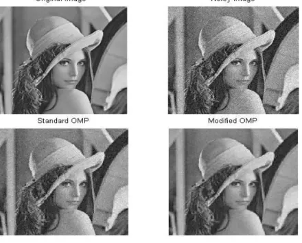
Fig 6 Experimental results (Lena Images)
Above figure shows the result of standard and modified OMP on the lena Image. The modified OMP image is clearer than the standard OMP image. The second and third image will validate this result further i.e. ‘The Boat’ Image and “Butterfly”.
Fig 7 : Experimental results (Boat Image) (a) Original Image (b) Noisy Image
(c) Standard OMP Image (d) Modified OMP image
(a) Original image (b)Noisy image
(c)Standard OMPimage (d)Modified image
Fig 8 Experimental Results (Butter fly image)
IV. CONCLUSION
The simulation results concludes that OMP performs better and slight improvement of 4 dB inPSNR has been observed for a single measurement value i.e. 80. Comparative analysis is made between BP and OMP based on the simulated results. It can be concluded that OPM is better than BP in terms of PSNR and an improvement by a factor of 2.5 is observed. comparison is made between BP and OMP in terms of computational time. It can be concluded that the computational time of OMP is less than that of BP by a factor of 2.Thus it is proved that OMP is faster as compared to BP in giving better results. Modified OMP gives better visual results as compared to standard OMP in presence of noise where sigma is 0.004 and compression ratio is 0.5.The computational times for OMP and Modified OMP are approximately same. It should also be noted that if any denoising technique is to be used for removal of noise from the recovered data of standard OMP, the computational time increases thus showing that the modified OMP is fast for recovering and denoising image at once.
V. REFERENCE
[1] B. F. Logan, “Properties of high-pass signals”, Ph.D. thesis, Columbia Univ., New York, 1965.
[3] D. L. Donoho and P. B. Stark, “Uncertainty principles and signal recovery”, SIAM J. Appl. Math 49 (1989), no. 3, 906-931.
[4] D. L.Donoho and B. F. Logan, “Signal recovery and the large sieve”, SIAM J. Appl.Math 52 (1992), no. 2, 577-592.
[5] An uncertainty principle for cyclic groups of prime order, Math. Res. Letters 12 (2005), 121-127
[6] J. F. Claerbout and F. Muir, “Robust modeling with erratic data”, Geophysics 38 (1973), no. 5, 826-844.
[7] L. I. Rudin, S. Osher, and E. Fatemi, “Nonlinear total variation noise removal algorithm”, Physica D 60 (1992), 259-268.
[8] H. L. Taylor, S. C. Banks, and J. F. McCoy, “Deconvolution with the l1 norm”, Geophysics 44 (1979), no. 1, 39-52.
[9] M. S. O'Brien, A. N. Sinclair, and S. M. Kramer, “Recovery of a sparse spike time series by l1 norm deconvolution”, IEEE Trans. Sig. Proc. 44 (1994), 3353-3365.
[10] Y. Wiaux, L. Jacques, G. Puy, A. M. M. Scaife, and P. Vandergheynst, “Compressed sensing imaging techniques for radio interferometry”, Mon. Not. R. Astron. Soc. 395 (2009), 1733-1742. [11] U. J. Schwarz, “Mathematical-statistical description of the iterative beam removing technique (method CLEAN)”, Astronomy &
Astrophysics (1978), 345.
[12] A. Papoulis and C. Chamzas, “Improvement of range resolution by spectral extrapolation”, Ultrasonic Imaging 1 (1979), no. 2, 121-135. [13] R. Mammone and G. Eichmann, “Restoration of discrete Fourier spectra using linear programming”, J. Opt. Soc. Am. 72 (1982), 987-992.
[14]CandèsEJ, “Compressive sampling”, International congress of mathematicians, vol.III .Zürich European Mathematical Society; 2006.p. 1433–52.
[15] M. Duarte, M. Davenport, D. Takhar, J. Laska, T. Sun, K. Kelly, and R. Baraniuk.“Single-pixel imaging via compressive sampling” IEEE Signal Processing Mag., 25(2):83-91, 2008.