Goussev, Oleg (2003): Non-LTE diagnostics of the infrared observations of the planetary atmosphere. Dissertation, LMU München: Fakultät für Physik

Non-LTE diagnostics of the

infrared observations

of the planetary atmosphere

Oleg Goussev

Non-LTE diagnostics of the

infrared observations

of the planetary atmosphere

Oleg Goussev

Dissertation

an der Fakultät für Physik

der Ludwig–Maximilians–Universität

München

vorgelegt von

Oleg Goussev

aus St. Petersburg

Table of contents

1 Introduction . . . 1

2 The non-LTE problem for molecular gas in the planetary atmosphere . . . 3

2.1 Formulation of the problem . . . 3

2.2 Complete thermodynamic equilibrium (CTE) . . . 5

2.3 Local thermodynamic equilibrium (LTE) . . . 5

2.4 Partial LTE . . . 7

2.4.1 Rotational LTE . . . 7

2.4.2 Vibrational LTE in groups of levels . . . 9

2.5 Ro-vibrational non-LTE . . . 10

3 Methods of solution of the non-LTE problem (current status) . . . 11

3.1 Lambda iteration . . . 11

3.2 Matrix method . . . 11

3.3 Comparison of lambda iteration and matrix method . . . 13

3.4 Accelerated lambda iteration . . . 14

3.5 Treating the nonlinearity arising from collisions . . . 15

3.5.1 Straightforward iteration and “decoupling” . . . 15

3.5.2 Newton–Raphson method . . . 16

4 Comparison of methods used to solve non-LTE problem in atmospheric science . . . 19

4.1 Comparison of the ALI and lambda iteration techniques . . . 19

4.2 Comparison of ALI algorithms utilising various radiative transfer techniques . . . 23

4.3 ALI–ARMS, MCM and ARC codes . . . 27

5 Applications of ALI-ARMS: non-LTE retrievals of the atmospheric parameters from CRISTA-1 and CRISTA-2 radiance data . . . 29

5.1 CRISTA-1 and -2 spectral channels with non-LTE emissions . . . 30

5.2 Method of retrieval . . . 33

5.3 Non-LTE retrieval of CO2densities . . . 35

5.4 Non-LTE retrieval of O3densities . . . 36

5.5 Non-LTE retrieval of temperature . . . 37

7 Applications of ALI-ARMS: vibration-rotational non-LTE in CO2 in the Earth

atmos-phere . . . 53

8 Conclusions . . . 57

9 Appendixes . . . 59

A Using spectral line databases for non-LTE studies . . . 61

A.1 Using HITRAN for non-LTE applications . . . 61

A.1.1 Line profiles and frequency quadrature scheme . . . 64

A.2 Definitions of vibrational temperature . . . 67

B Electronic-vibrational-rotational levels and bands of molecules used in this study . . 71

B.1 H2O . . . 71

B.2 CO2 . . . 72

B.3 O3 . . . 73

B.4 N2O . . . 75

B.5 CO . . . 75

B.6 O2 . . . 76

B.7 N2 . . . 77

C Collisional rates . . . 83

C.1 R−Tcollisional processes . . . 83

C.1.1 Rate coefficients for the CO2R−Tenergy exchange . . . 83

C.2 V−Tcollisional processes . . . 83

C.2.1 V−Tcollisional transitions in H2O . . . 83

C.2.2 V−Tcollisional transitions in CO2 . . . 84

C.2.3 V−Tcollisional transitions in O3 . . . 86

C.2.3.1 Kinetic model of Manuilova . . . 87

C.2.3.2 Kinetic models of Mlynczak . . . 88

C.2.3.3 Kinetic model of Koutoulaki . . . 88

C.2.4 V−Tcollisional transitions in N2O . . . 89

C.2.5 V−Tcollisional transitions in CO . . . 90

C.2.6 V−Tcollisional transitions in N2 . . . 90

C.2.7 V−Tcollisional transitions in O2 . . . 90

C.3 V−Vcollisional processes . . . 91

C.4 C−Vprocesses . . . 95

C.4.1 Production of ozone: recombination reaction . . . 95

Table of contents VII

C.4.3 Destruction of ozone by reactions with other minor chemical species . . . . 97

C.4.4 Chemical excitation of O2 . . . 97

D Solution of the radiative transfer equation (RTE) . . . 99

D.1 Optical depth . . . 100

D.2 Lambda and psi operators . . . 100

D.3 Integral methods . . . 101

D.3.1 Method of long characteristics (MLC) . . . 101

D.3.2 Method of short characteristics (MSC) . . . 101

D.4 Differential methods . . . 102

D.4.1 Feautrier method . . . 102

D.4.2 Discontinuous finite element (DFE) method . . . 103

D.5 Treating laser bands . . . 104

D.6 Comparison of the methods . . . 105

E Numerical acceleration techniques . . . 107

E.1 Ng acceleration . . . 107

E.2 Orthomin acceleration . . . 108

F Atmospheric models used in this study . . . 109

F.1 Earth atmosphere . . . 109

F.1.1 Pressure and temperature . . . 109

F.1.2 Volume mixing ratios . . . 110

F.2 Mars atmosphere . . . 111

F.2.1 Mars and Earth atmospheres: the comparison . . . 113

G Current status of the code package ALI-ARMS (technical details) . . . 115

G.1 General features of the code . . . 115

G.2 Possible future extensions . . . 116

G.3 Implemented models . . . 116

H The non-LTE problems for various molecules in the Earth atmosphere solved by ALI-ARMS . . . 119

H.1 Vibrational non-LTE in CO2 . . . 119

H.2 Vibrational non-LTE in O3 . . . 120

H.3 Vibrational non-LTE in H2O . . . 123

H.4 Vibrational non-LTE in N2O . . . 124

H.5 Vibrational non-LTE in CO . . . 126

H.7 Vibrational non-LTE in N2 . . . 128

Acknowledgements . . . 131

Lebenslauf . . . 133

Abbildungsverzeichnis

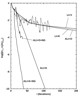
4.1 Convergence plots for the 9-level CO2 model of a spring equinox atmosphere at

night. Logarithms of the maximum absolute relative change (MARC) are presented for the 00011 CO2level. Labels on the curves refer to various iteration schemes (LI,

LI+V, etc); use of Ng’s acceleration method indicated by (+NG). . . 20

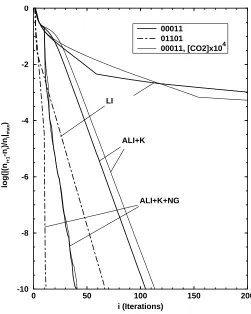
4.2 Convergence plots for the 9-level CO2 model of a spring equinox atmosphere at night. Logarithms of MARC are presented for the 00011 and 01101 CO2levels (thick solid and dashed curves) . . . 22

4.3 Convergence plots for a 64-level CO2 model of a spring equinox atmosphere for night and for day conditions (at solar zenith angle 0◦). . . 23

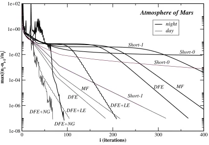
4.4 Convergence plots for the CO2 problem in the Martian atmosphere for day and night conditions. Labels on the curves refer to various iteration schemes (see text for details). . . 25

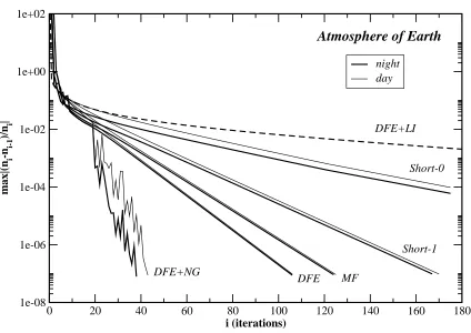
4.5 Convergence plots for the CO2 problem in the Earth’s atmosphere for day and night conditions. Labels on the curves refer to various iteration schemes (see text for details). . . 26

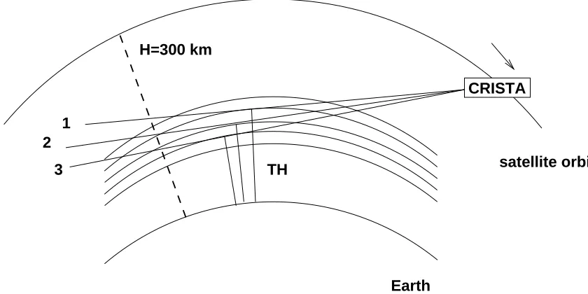
5.1 The geometry of limb scanning (CRISTA flight parameters used) . . . 29

5.2 The measured limb spectra in the SCL2 CRISTA channel . . . 31

5.3 The simulated spectra in the SCL2 CRISTA channel at different tangent heights . . 32

5.4 The simulated spectra in the SCS8 CRISTA channel at different tangent heights (daytime) . . . 33

5.5 The simulated spectra in the SCS8 CRISTA channel at different tangent heights (nighttime) . . . 34

5.6 The measured daytime limb spectra in the SCS2 CRISTA channel at different tan-gent heights . . . 39

5.7 The simulated spectra in the SCS2 CRISTA channel at different tangent heights (daytime) . . . 40

5.8 The simulated spectra in the SCS2 CRISTA channel at different tangent heights (nighttime) . . . 40

5.9 The measured limb spectra in the SCS3 CRISTA channel (day/night) . . . 41

5.10 The simulated spectra in the SCS3 CRISTA channel at different tangent heights (nighttime) . . . 42

5.11 The simulated spectra in the SCS3 CRISTA channel at different tangent heights (daytime) . . . 42

5.12 CO2volume mixing ratios. . . 43

5.13 Integrated limb radiances in the SCS2 channel for selected CO2profiles . . . 43

5.14 Retrieved CO2VMR for selected CRISTA-1 profiles. . . 44

5.16 The profiles of retrieved non-LTE O3VMR, the LTE retrieved O3VMR and the MAS

measurement . . . 45

5.17 Zonal averages of the temperature (top: CRISTA-1, bottom: CRISTA-2 extended scans). The latitude binning is 10◦in both cases. . . 46

5.18 The zonal temperature cross-section (bottom: CRISTA-1, top: CRISTA-2). . . 47

6.1 The vibrational temperatures for CO2(626) levels (daytime). . . 49

6.2 The vibrational temperatures for CO2(626) levels (nighttime). . . 49

6.3 The temperatures in Mars atmopshere and on its surface, measured by MGS/TES. 50 6.4 Global distribution of the emissions in CO2 10µm laser band: modelled (contour lines) and measured by MGS/TES.The figure is taken fromMaguire et al.(126). . . . 51

7.1 The rotational distribution functions for the vibrational level 00011 of CO2(626) at different altitudes . . . 55

7.2 The nighttime limb radiances for the CO2 (626) 00011 →00001 band at different tangent heights. Effects of the rotational LTE breakdown. . . 56

A.1 Dependence of Einstein coefficient of spontaneous emission for the vibrational band on temperature (in case of rotational LTE). . . 63

A.2 The populations of the ground vibrational state . . . 67

B.1 The vibrational levels and most important 6.3µm (solid lines) and 2.7µm (dashed lines) bands of H2O . . . 72

B.2 Energies of H2O vibrational levels, cm−1 . . . 72

B.10 The vibrational levels and bands of CO . . . 75

B.11 Energies of CO vibrational levels, cm−1 _{. . . . 75}

B.3 The vibrational levels of CO2(extended model). . . 78

B.4 Vibrational bands of CO2: black - 15µm , red - 10µm , blue - 4.3µm , magenta - 2.0 µm . . . 79

B.5 The vibrational levels of O3(taken fromKoutoulaki(92)). . . 80

B.6 The vibrational levels of O3included in the model ofManuilova et al.(132). . . 80

B.7 Most important 4.8µm (left) and 9.6µm (right) bands of O3 . . . 81

B.8 The vibrational levels and bands of N2O . . . 81

B.9 Energies of N2O vibrational levels . . . 81

C.1 Most importantV−Vprocesses. . . 91

C.2 Rate constants for O2(v)+O2(0) process. . . 95

C.3 V−Vrate constants for O2(v)+N2(0) process. . . 95

C.4 Chemical production rate constant of O2(3Σ,v) from O3 . . . 98

ABBILDUNGSVERZEICHNIS XI

F.1 Altitude profiles of pressure and temperature, used for the Earth atmosphere

mo-deling. . . 109

F.2 Altitude profiles of molecular VMRs used for the Earth atmosphere modeling. . . 110

F.3 Altitude profiles of molecular VMRs used for the Earth atmosphere modeling (cont.)111 F.4 Altitude profiles of pressure and temperature, used for the modeling of Mars at-mosphere. . . 112

F.5 Volume mixing ratio of CO2in Mars atmosphere . . . 112

F.6 Volume mixing ratio of N2in Mars atmosphere. . . 112

F.7 Volume mixing ratio of CO in Mars atmosphere . . . 112

F.8 Volume mixing ratio of O(3_P J)in Mars atmosphere. . . 112

F.9 Altitude profiles of pressure and temperature, used for the Earth and Mars atmos-pheres . . . 113

F.10 Altitude profiles of CO2number density in the Earth and Mars atmospheres . . . . 113

H.1 The vibrational temperatures for CO2(626) levels (daytime). . . 119

H.2 The vibrational temperatures for CO2(626) levels (nighttime). . . 119

H.3 The convolved limb radiances of CO2 15, 12.6, 9.4, 4.3 µm bands (only daytime profiles are shown) . . . 120

H.4 The cooling rates for CO2(626) molecule . . . 121

H.5 The cooling rates for CO2(636) molecule . . . 121

H.6 The vibrational temperatures for O3(666) levels (daytime). . . 121

H.7 The vibrational temperatures for O3(666) levels (nighttime). . . 121

H.8 The convolved limb radiances of O39.6µm bands (daytime) . . . 122

H.9 The convolved limb radiances of O39.6µm bands (nighttime) . . . 122

H.10 The convolved limb radiances of O34.8µm bands (nighttime) . . . 122

H.11 The cooling rate for O3molecule . . . 123

H.12 The vibrational temperatures for H2O (161) levels (daytime). . . 123

H.13 The vibrational temperatures for H2O (161) levels (nighttime). . . 123

H.14 Daytime convolved limb radiances of 6.3µm H2O bands. . . 124

H.15 Nighttime convolved limb radiances of 6.3µm H2O bands. . . 124

H.16 The cooling rate for H2O molecule . . . 125

H.17 The vibrational temperatures for N2O (446) levels (daytime). . . 125

H.18 The vibrational temperatures for N2O (446) levels (nighttime). . . 125

H.19 The vibrational temperatures for CO (26) levels (daytime). . . 127

H.20 The vibrational temperatures for CO (26) levels (nighttime). . . 127

H.21 The convolved limb radiances of CO24.7µm bands . . . 127

H.22 The cooling rate for CO molecule . . . 128

H.24 The vibrational temperatures for O2(66) levels (nighttime). . . 128

H.25 The vibrational temperatures for N2(44) levels (daytime). . . 129

Tabellenverzeichnis

5.1 Spectral channels of CRISTA-1 and -2. The /E denotes the CRISTA-2 extended

channels. . . 30

5.2 CRISTA-1 and -2 spectral channels with the non-LTE emissions. . . 31

A.1 Molecular parameters (source - HITRAN-2000) . . . 69

B.1 Energies of O3vibrational levels . . . 74

B.2 Energies of O2electronic states. The values are in cm−1. . . 76

B.3 Constants used for the calculation of vibrational energies of O2 . The values are taken fromLaher and Gilmore(105) andHerzberg(77). . . 76

B.4 Constants used for calculation of rotational energies of O2 . The values are taken fromHerzberg(77) in cm−1_{. . . . 77}

B.5 Constants used for the calculation of vibrational energies of N2. The energies are in cm−1 _{. . . . 77}

B.6 Constants used for calculation of rotational energies of N2. The values are in cm−1 77 C.1 V−Trate constants for H2Oν2transitions. . . 84

C.2 V−Trate constants for H2Oν1 ↔ν3exchange. . . 84

C.3 V−Trate constants for H2Oν1,ν3 ↔2ν2exchange. . . 84

C.4 Rate constants for theV−Tprocesses, which lead to splitting of thev3 quantum of CO2molecules. . . 85

C.5 V−Trate constants for CO2v2quenching. . . 85

C.6 V−Trate constants for CO2transitions inside then-family. . . 86

C.7 Branching ratiosnlfor CO2v3splitting. . . 86

C.8 V−Trate constants for O3ν1↔ν3transitions. . . 87

C.9 V−Trate constants for O3ν1↔ν2andν3↔ν2transitions. . . 87

C.10V−Trate constants for O3ν2transitions. . . 87

C.11V−Trate constants for O3O(3PJ)quenching. . . 88

C.12 ParametersAandBused byKoutoulaki(92). . . 88

C.13 Averaged collisional rates used byKoutoulaki(92) . . . 89

C.14V−Tprocesses for N2Oν2bending mode. . . 89

C.15V−Trate constants for O2(3Σ,v) quenching. . . 90

C.16 Rate constants for N2(v)+N2(0) process . . . 95

C.17 Rate constants of O3chemical production . . . 96

Zusammenfassung XV

Zusammenfassung

Für die Analyse der Infrarotmessungen von mehreren Weltraumexperimenten benötigt man die Berechnung der molekularen Infrarotstrahlung unter Berücksichtigung des nichtlokalen thermo-dynamischen Gleichgewichts (non–LTE). In dieser Dissertation wird die allgemeine Formulie-rung des non-LTE-Problems für die Mischung molekularer Gase in einer Planetenatmosphäre gegeben. Die hier vorgeschlagene Methode für die Lösung dieses Problems verwendet die ”Ac-celerated Lambda Iteration (ALI)”, die in der Astrophysik für die non-LTE Modellierung der Sternatmosphären entwickelt worden ist. Diese für die Atmosphärenforschung neue Technik ist frei von den Beschränkungen der Matrix- und Lambda-Iterationsmethoden, mit denen man tradi-tionell die non-LTE Probleme in den Planetenatmosphären behandelt. Mit der Lösung des CO2

-non-LTE Problems in der Erd- und Marsatmosphäre wird demonstriert, dass die ALI-Methode den anderen Algorithmen in Rechenzeit und Arbeitsspeicherverbrauch weit überlegen ist. Wäh-rend sich die Atmosphärengruppen auf die Lösung einiger ausgewählter non-LTE-Probleme be-schränkten, erlaubt das im Rahmen dieser Studie entwickelte Computerprogramm ALI-ARMS (für “Accelerated Lambda Iteration for Atmospheric Radiation and Molecular Spectra”) die non-LTE-Modellierung einer beliebigen Anzahl von Molekülen, die durch den Stoß- und Strahlungs-austausch von Energie gekoppelt sind. ALI-ARMS wurde angewandt für die Datenauswertung der Infrarotspektren, die von dem “CRyogene Infrarot-Spektrometer und Teleskope für die Atmo-sphäre (CRISTA)”-Experiment an Bord des deutschen ASTRO-SPAS-Satelliten gemessen wurden, und für die Analyse der 10µm Laser Banden, die von dem Thermal Emission Spectrometer (TES) an Bord von Mars Global Surveyor (MGS) aufgenommen wurden. Im Fall der Erdatmosphäre wurden die ersten detaillierten Karten der Temperatur sowie der Spurengaskonzentrationen in der oberen Mesosphäre und untereren Thermosphäre erzeugt. Die Ergebnisse dieser Arbeit sind ein wesentlicher Beitrag zu Studien der Mesosphäre, die heute als Indikator der globalen Klima-veränderungen betrachtet wird.

Abstract

The analysis of the infrared measurements of a number of sophisticated space experiments re-quires modeling of molecular infrared radiation with accounting for the nonlocal thermodyna-mic equilibrium (non–LTE). In this dissertation a general formulation is given of the multilevel vibrational-rotational non-LTE problem for a mixture of radiating molecular gases in a planetary atmosphere. The approach for the solution of this problem suggested here utilizes the Accelerated Lambda Iteration (ALI) technique developed in stellar astrophysics for spectrum formation calcu-lations and for the computation of non-LTE model stellar atmospheres. This new for atmospheric science technique is not subject to the limitations of the traditional matrix and conventional lamb-da iteration methods which dominate the studies dealing with non-LTE in planetary atmospheres. In the case of the CO2 non-LTE problems in the atmospheres of Earth and Mars it is

1. Introduction

Adequate interpretation of the infrared space observations of the Earth’s and planetary atmos-pheres plays an important role in the comparative analysis of the planetary atmosatmos-pheres which is aimed at understanding of possible evolution ways of the Earth’s ecosystem.

In recent years the observations of infrared molecular emissions from the middle and upper layers of the Earth’s atmosphere have attracted particular attention since trends in this altitude region are significant for understanding of global changes of the atmosphere. Simultaneously a number of sophisticated ground based and space infrared experiments provided unique data about the upper planetary atmospheres. However, an essential problem here is that in many cases the in-terpretation of these data requires accounting for deviations from the local thermodynamic equi-librium (non-LTE). The non-LTE effects are crucial in the middle and upper Earth’s atmosphere for the majority of infrared molecular bands and influence strongly the radiation emerging from these layers. In some cases the observations of these emissions from space are influenced by the non-LTE effects down to the lower stratosphere.

The non-LTE problems for the infrared ro-vibrational molecular bands are studied in atmospheric science since 1950s. Any of these problems has two primary constituents: (1) the statistical equi-librium equations (SEE), which express the equality of the total population and de-population rates for each molecular level; (2) the radiative transfer equation (RTE), which relates the radia-tion field at a given hight to the level popularadia-tions atall altitudes in the atmosphere. Hence the system of equations for the level populations isnonlocal(and nonlinear).

The most obvious way of dealing with this situation is to iterate between the SEE and RTE (see

Wintersteiner et al.(219),López-Puertas and Taylor(121)). This process, traditionally called “lambda iteration”, has been investigated in detail in the astronomical context in the 1920’s (c.f. Unsöld(206)). It involves matrices no larger thanL×L, whereLis the total number of molecular levels, but in some cases (if the optical depths are large) it converges very slowly.

An alternative way of dealing with this non-LTE problem is the simultaneous treatment of the SEE and RTE, in which the RTE is discretized with respect to the optical depth or pressure grid to get a matrix representation of the radiative terms in the SEE. This requires the inversion of a matrix of dimension(L×D)×(L×D), whereDis the number of altitude (or pressure) points in the atmospheric model. This approach is known in atmospheric science as the Curtis-matrix technique (see Curtis and Goody(34), Goody(63)). It has been employed in a series of papers beginning withLópez-Puertas et al.(109) (see alsoLópez-Puertas and Taylor(121) ).

However, in order to construct adequate models, one must consider a large number of exited le-vels of different molecular species coupled by a variety of collisional energy exchange processes and by band overlapping, together with a detailed model of atmospheric stratification; thus both

LandDcan become large. The dimensions of the primary matrices were consequently reduced by introducing approximations; these, however, need careful investigation, since in many cases they lead to unrealistic results. Typical of these are: 1) the assumption of rotational LTE for rota-tional substructures of vibrarota-tional levels, which reducesLto the number of vibrational levels; 2) the assumption of vibrational LTE for groups of vibrational levels closely spaced in energy and interacting by intensive inter- or intra-molecular collisional V-V energy exchange; 3) the neglect of certain vibrational levels or exclusion from the model of certain molecules. Moreover, in many cases a large number of weak bands are omitted or treated approximately, the total number of molecules is not conserved, etc.

developed (seeHubený et al.(80) ) a family of powerful techniques, which utilize iteration with an approximate (or accelerated) lambda operator; these are now the standard techniques for spec-trum formation calculations and for the computation of non-LTE model stellar atmospheres. In these so-called ALI techniques (for Accelerated Lambda Iteration) the lambda operator, which express the radiation intensity at a point in terms of the level populations at all points, is appro-ximated by a local (or nearly local) operator and thedifference is treated iteratively. Again, the largest matrix has dimensionL×L, but the convergence is now rapid.

The Chapter 2 of this dissertation gives general formulation of the multilevel vibrational-rotational non-LTE problem for a mixture of radiating molecular gases in a planetary atmosphere. Chapter 3 contains description and comparative analysis of conventional lambda iteration-, matrix- and ALI techniques. The ALI-ARMS (for “Accelerated Lambda Iteration for Atmospheric Radiation and Molecular Spectra”) code developed in framework of this study utilizes newest results of the ALI techniques obtained in the stellar astrophysics. Chapter 4 gives the convergence rates and timing of various computational schemes based on accelerated lambda iteration which are incor-porated in the code, as well as compares the code with other codes currently used in atmospheric non-LTE studies. In the last three Chapters the application of ALI-ARMS are discussed. Chapter 5 outlines results of the non-LTE diagnostics of the limb radiance data obtained in the CRyoge-nic Infrared Spectrometers and Telescopes for the Atmosphere (CRISTA) experiments on board of the german ASTRO-SPAS satellite. Chapter 6 deals with the analysis of the limb radiance da-ta of the Thermal Emission Spectrometer (TES) instrument orbiting Mars on board of the NASA Mars Global Surveyor (MGS) satellite. Chapter 7 presents analysis of the rovibrational non-LTE in CO2in the Earth’s middle atmosphere. In the conclusion the main results and implications of

2. The non-LTE problem for molecular gas in the planetary

atmosphere

2.1 Formulation of the problem

Let us consider a Maxwellian gas mixture in a planetary atmosphere consisting of molecular and atomic gases whose energy levels are enumerated by the indexlthroughout the entire mixture. Each energy level is characterized by its statistical weightgland energyEl.

We consider only thesteady stateof this gas mixture, in which its temperature and the degree of excitation do not change with time. The statistical equilibrium (or steady-state) equation (SEE) which expresses the balance between various elementary processes can be written as

nl

∑

l0

Rll0+C→_l

=

∑

l0

nl0R_l0_l+C←_l +Y_l. (2.1)

Herenl are the populations of electronic–vibration–rotational (EVR) levels of the molecules or

the electronic (E) levels of atoms,Rll0 are the radiative rate coefficients for transitions from level ltol0,nlCl→ andC←l are the total rates of de-population and population of levell, respectively,

due to the variety of energy exchange processes by atomic and molecular collisions.Ylin Eq. 2.1,

(p. 3) is a source term prescribing the net production rate of levellthrough processes other than collisions and absorption of radiation emitted within the atmosphere, such as the absorption of radiation from external sources (“sun” and/or “ground”), production of excited constituents in various chemical reactions, etc.

For the sake of simplicity we confine ourselves to the case of a plane-parallel atmosphere for which the transfer equation is

µdIµν

dz =−χµ(ν)Iµν+ηµ(ν), (2.2)

where Iµν is the specific intensity of atmospheric radiation, and χµ(ν)and ηµ(ν) are the total opacity and emissivity, respectively, at frequencyνand direction cosineµ.

The radiative properties of the gas being considered are completely characterized by the emissi-vityη_ll0 and the opacityχ_ll0 for each pair of levels connected by a line transition1. If the

macros-copic velocity field can be neglected, which is obviously a good approximation for any molecular radiative transfer problem in planetary atmospheres, these quantities do not depend onµ. Abbre-viating the energy relationsEl < El0 andE_l >E_l0 byl ≺l0andl l0, respectively, we obtain for ll0

ηll0(ν) = h

νll0

4π nlAll0ϕll0(ν), χ_ll0(ν) = h

νll0

4π (nl0Bl0l−nlBll0)ϕll0(ν),

(2.3)

whereνll0 is the line center frequency,A_ll0,B_ll0 andB_l0_l are the Einstein coefficients andϕ_ll0(ν)is

the line profile function normalized such thatR

dνϕll0(ν) = 1. The line source function for the

transition is defined by

Sll0 =

ηll0(ν)

χ_ll0(ν) =

nlAll0

nl0B_l0_l−n_lB_ll0. (2.4)

It is frequency and angle independent as a result of assuming in Eq. 2.3, (p. 3) the equality of emission and absorption profiles (the assumption of complete frequency redistribution within

a line) and isotropic scattering. Generalizations to include angle and frequency variations are available, but will not be considered here.

The total emissivity and opacity are given in terms of above line quantities by

η(ν) =

∑

ll0

ηll0(ν) +η_c(ν),

χ(ν) =

∑

ll0

χ_ll0(ν) +χ_c(ν),

(2.5)

where ηc(ν) and χc(ν) are the emissivity and opacity of the background continuum which is

slowly varying across the line; these quantities are assumed to be prescribed and do not change from iteration to iteration. In writing Eq. 2.3, (p. 3) we ignored the processes of monochromatic scattering of photons such as Rayleigh scattering or scattering due to aerosol particles which can be important for certain atomic transitions and some molecular near-infrared bands in planetary atmospheres. Finally, the total source function is then

Sν =

η(ν)

χ(ν). (2.6)

The radiative rate coefficients in SEE Eq. 2.1, (p. 3) are given by

Rll0 =A_ll0+B_ll0J¯_ll0 (2.7)

for bothl l0 andl ≺ l0(since in latter case All0 ≡ 0), where ¯J_ll0(= J¯_l0_l)is the integrated mean

intensity, defined by

¯

Jll0 = 1

4π

Z

dΩ

Z

dνϕ_ll0(ν)I_µν. (2.8) Cl→ in Eq. 2.1, (p. 3)describes the total loss rate for the level l (per its unit population) due to

collisionally induced energy transfer processes. It is written as

C→l =

∑

l0

Cll0+

∑

l0_,`,`0

n`Cll0_,``0. (2.9)

The first term here defines the rate of electronic–vibration–rotational energy transfer to the trans-lational energy (EVR–T). In it

Cll0 =

∑

β

nβ_kβ

ll0, (2.10)

wherekβ_ll0are rate constants for EVR–T transitionl→l0by the collisions with molecules or atoms

ofβ-constituent of gas mixture with total densitynβ_.

The second term in Eq. 2.9, (p. 4) describes the loss rate of levellvia the processes of EVR–EVR energy exchange. ThereCll0_,``0 are rate coefficients for the transitionsl→l0in one and the

transi-tions`→`0in another of two colliding molecules and/or atoms.

Accounting for Eq. 2.9, (p. 4), we can write the termC_l←in the right–hand side of Eq. 2.1, (p. 3) as

Cl←=

∑

l0

nl0C_l0_,l+

∑

l0_,`,`0

nl0n_{`</sub>0C<sub>l</sub>0<sub>l,`}0_`. (2.11)

The collisional rate coefficients in Eq. 2.9, (p. 4)-Eq. 2.11, (p. 4) are related by the obvious detailed balance expressions

n∗lCll0 =n∗

l0C_l0_l and n∗

ln

∗

`Cll0_,``0 =n∗

l0n∗_{`</sub>0C<sub>l</sub>0<sub>l,`}0_`, (2.12)

wheren∗_l are the LTE populations.

Since the RTE Eq. 2.2, (p. 3)relates the radiation field at a given hight to the level populations at

all altitudesin the atmosphere, the SEE system Eq. 2.1, (p. 3)for the level populations is nonlocal

2.2 Complete thermodynamic equilibrium (CTE) 5

coefficients Eq. 2.10, (p. 4)do not introduce non-linearity in SEE. However, the additional (local) non–linearity enters SEE through the second terms inC→_l andC_l←which deal with the processes of EVR–EVR energy exchange.

The non–LTE problem for the gas in the planetary atmosphere formulated above is aimed at utmost detailed description of molecular bands. In the majority of applications those are infra-red or near-infrared bands related to vibrational levels of electronic ground states of molecules. Also some electronically excited atoms produced in the photo-chemical reaction are usually involved due to the importance of collisional transfer of electronic energy to molecular vibrations. The number of these atomic states is limited. However, the total number of levels in the problem can be very large (up to a few thousands) because of the large number of rotational sublevels of vibrational levels required to be accounted for the adequate description of bands.

Now let us look in more detail at several special steady states of the gas. We will follow here the discussions byIvanov(84) and Mihalas (139) of similar situations for an atomic gas in the astrophysical context.

2.2 Complete thermodynamic equilibrium (CTE)

In this state the velocity distribution of molecules is Maxwellian, the level populations obey the Boltzmann law

nl0 nl

= gl0

gl

exp−El0−El kT

(2.13) and the radiation intensity is isotropic, unpolarised, homogenous and is given by the Planck func-tion. Only one parameter - the temperatureT- completely determines this state. Moreover, in CTE all processes obey the principle of detailed balance: each process is exactly compensated by its in-verse. In particular, the number of radiative transitions from an upper levell to a lower levell0

then is equal to the number ofl0 →lradiative excitations

nl(All0+B_l,l0J¯_ll0) =n_l0B_l0_lJ¯_ll0. (2.14)

Here ¯Jll0is the radiative mean intensity at the line center frequencyν_ll0

hν_ll0 =E_l0−E_l. (2.15)

It follows from Eq. 2.13, (p. 5) and Eq. 2.14, (p. 5) that ¯

Jll0 =B_ν

ll0(T) =2hcν 3

ll0

h

exphνll0

kT

−1i

−1

(2.16) is also the Planck function.

For collisional transitions the detailed balance relation has the form

nl0C_l0_l =n_lC_ll0, (2.17)

or with the accounting for Eq. 2.13, (p. 5)

Cl0_l=C_ll0 gl gl0 exp

− El−El0 kT

. (2.18)

2.3 Local thermodynamic equilibrium (LTE)

We now assume that the index l corresponds to the pair of indices v j, which specify the ro-vibrational state of molecule; herevand jare the indices of a vibrational level and its rotational sub-level, respectively. For a triatomic linear molecule, for instance,vrepresents the combination of four indicesv1vl

2v3 specifying the vibrational state, therefore the sums over this index in our

treatment imply summation over all available combinations of these four indices.

LTE is the state of the gas in which the velocity distribution of molecules is Maxwellian, popu-lations follow the Boltzmann distribution, while the radiation intensity is not, in general, given by Planck function. Such a state can exist when both radiative and external source terms in the SEE are small in comparison to the collisional terms. If the velocity distribution of all molecules is Maxwellian then the detailed balance relations Eq. 2.17, (p. 5) are still valid. If one now neglects all radiative terms as well as the source terms in the SEE, these equations reduce to the Boltz-mann law. Since these equations are linear in the quantitiesnv j, the equilibrium populations are

in fact the only solution. The temperature in the Boltzmann relation may now change from point to point. A Maxwellian gas is also in LTE in those layers where the external source terms in the SEE are small compapred to collisional terms and the radiative terms dominate the collisional terms but cancel each other according to the relations (Eq. 2.14, (p. 5)). This occurs, for instance, for optically thick transitions in deep atmospheric layers.

Let us now introduce the population probabilityWv jof a ro-vibrational levelv jof a specific

mo-lecular specieα, such that

Wv j=

nv j

nα, (2.19)

wherenα_{is the number density of specie in question. All the LTE values later on will be marked} with the star symbol (∗) . Accounting for the Boltzmann relation (Eq. 2.13, (p. 5)) one can easily derive that

Wv j∗ =

gv j

Q∗_(T)exp

−Ev j kT

, (2.20)

where

Q∗(T) =

∑

v j

gv jexp

− Ev j kT

(2.21) is the total ro-vibrational internal sum, so that

∑

v j

Wv j∗ =1. (2.22)

One can also introduce the probabilityWvthat the molecule is in the vibrational statev

nv=

∑

j

nv j=nαWv, (2.23)

wherenvis the population of vibrational levelv. Deriving the expression forWvtwo facts should

be considered

1. the energy of the ro-vibrational level may be expressed as the sum

Ev j =Ev+Ej,v (2.24)

of the vibrational energyEvof statevand the rotational energyEj,v,

2. the statistical weight of the ro-vibrational level is the product

gv j =gvgv(j) (2.25)

of the statistical weight gv of vibrational level vand the degeneracygv(j)of its rotational

2.4 Partial LTE 7

Accounting for Eq. 2.20, (p. 6), Eq. 2.21, (p. 6), Eq. 2.24, (p. 6) and Eq. 2.25, (p. 6) one can derive that

Wv∗ =gvQ

∗

v(T)

Q∗_(T)exp

− Ev kT

, (2.26)

where

Q∗v(T) =

∑

gv(j)exp

−Ej,v kT

(2.27) is the rotational partition sum for the vibrational levelv. Finally, introducing the population pro-bability

Wv∗(j) =

gv(j)

Q∗

v(T)

exp−Ej,v kT

(2.28)

of the rotational subleveljof levelv, one may rewrite Eq. 2.20, (p. 6) as

Wv j∗ =W

∗

vW

∗

v(j). (2.29)

It follows from Eq. 2.23, (p. 6) and Eq. 2.26, (p. 7) that the LTE populations of two vibrational levels

vandv0are related as

n∗v0 n∗ v = W ∗ v0 W∗ v

= gv0

gv

exp− Ev0−Ev kT

Q∗

v0(T)

Q∗

v(T)

. (2.30)

2.4 Partial LTE

The gas is said to be in a non-LTE state when the level populations do deviate from the Boltzmann law while the molecular velocity distribution remains Maxwellian. One may describe this state with the same probability formalism as was used above for the case of LTE by introducing at each point a set of excitation temperatures instead of the one parameterT.

The complete LTE or non-LTE are hardly ever encountered in planetary atmospheres. In reality the gas is mainly in a state that might be calledpartial LTEin which the velocity distribution of molecules is Maxwellian but only some groups of levels obey the Boltzmann relation (Eq. 2.13, (p. 5)). If one considers a certain volume of gas and traces its state as the density decreases, then generally one will observe a series of the partial LTE states, in which ever fewer levels follow the Boltzmann relation. Two such states are discussed, which are of special importance.

2.4.1 Rotational LTE

If the gas density is relatively high, the collisional processes dominate the excitation of molecules and the level populations are in LTE. As the density decreases the most highly excited vibrati-onal levels are the first to depart from the Boltzmann law. This occurs sinceV−T and V−V

collisional processes are no longer able to maintain the coupling of these levels with the therma-lized levels against the influence of non-Planckian radiative transitions. As the density decreases further, departures occur for ever lower vibrational levels. However, within a wide range of den-sities the collisional processes between the rotational levels (R−T) can still keep the rotational substructure of all vibrational levels thermalized. This state of the gas may be described by means of probabilities as follows

Wv j=WvWv∗(j). (2.31)

HereW∗

v(j)is still given by Eq. 2.28, (p. 7), whileWvhas now the form

Wv=gv

Q∗

v(T)

Q exp

− Ev kTv

with Tv = Tfor vibrational levels which remain in the equilibrium and with Tv 6= T for those

which do not.Q, which replacesQ∗in Eq. 2.32, (p. 7), is the total internal sum

Q=

∑

v

gvexp

− Ev kTv

Q∗v(T) (2.33)

and is no longer a function of a single parameterT.

The state of the gas described above is a typical example of a partial LTE state and is usually called vibrational non-LTE with an assumption that the rotational substructure of all vibrational levels is thermalized, i.e. is in rotational LTE. Since theW∗

v(j)are known for each vibrational level

v, then only the populationsnv are to be found, thus reducing greatly the number of unknown

variables. The corresponding SEE is the sum overjof the Eq. 2.1, (p. 3). Since transitions between the sublevelsjof vibrational levelvcan not change the total population of this levelnv, the sums

of corresponding terms in Eq. 2.1, (p. 3) cancel. Then, accounting for Eq. 2.31, (p. 7), instead of the system Eq. 2.1, (p. 3), one obtains

nv

∑

v0

Rvv0+C→

v

=

∑

v0

nv0R_v0_v+C←

v +Yv. (2.34)

Here

Rvv0 =

∑

j,j0

Wv∗(j)Rv j,v0_j0 = A_vv0(T) +B_vv0(T)J¯_vv0, (2.35)

Avv0(T) =

∑

j,j0

Wv∗(j)Av j,v0_j0 (2.36)

is the de-excitation rate per molecule in the vibrational statev for spontaneous emission in the ro-vibrational bandv → v0(for v < v0 Avv0 ≡ 0); B_vv0(T)and B_v0_v(T)are related to A_vv0(T)by

expressions

Avv0 =2hcν3_vv0B_vv0, g_vB_vv0 =g_v0B_v0_v; (2.37)

whereνvv0, defined as

hνvv0 =E_v−E_v0 (2.38)

is the frequency of vibrational transition;Bvv0J¯_vv0is the de-excitation (stimulated emission) or

ex-citation (absorption) rate for the ro-vibrational bandv→v0per molecule in statev; the termsCv→

and C←v have the same structure as the corresponding terms in Eq. 2.1, (p. 3), however involve

vibrational populations and collisional rate coefficients for V–T transitions between vibrational levels

Cvv0(T) =

∑

j,j0

Wv∗(j)Cv j,v0_j0 (2.39)

and rates of V–V transitions (see detailed discussion of these terms in Section 3.5 (p. 15)) ¯

Jvv0in Eq. 2.35, (p. 8) has the form

¯

Jvv0 = 1 Bvv0

∑

j,j0

Wv∗(j)Bv j,v0_j0J¯_{v j,v}0_j0. (2.40)

It replaces ¯Jll0 in similar expression (Eq. 2.7, (p. 4)) for the radiative rate coefficients for a single

line and has, therefore, the meaning of the integrated mean intensity in the ro-vibrational band. Note that Eq. 2.34, (p. 8) for vibrational level populations have the same form as Eq. 2.1, (p. 3) for the ro-vibrational populations in which the integrated mean intensities for single lines ¯Jll0, Eq. 2.8,

(p. 4) are replaced by ¯Jvv0 for bands and where A_vv0(T)andB_vv0(T)enter as the effective

(tempe-rature dependent) Einstein coefficients for vibrational transitions. This tempe(tempe-rature dependence results from summation the temperature independent coefficientsAv j,v0_j0 for ro-vibrational

tran-sitions with the temperature dependent weighting functionW∗

v(j), Eq. 2.28, (p. 7).

The detailed balance relation forCvv0is now Cvv0

Cv0_v

= gv0

gv

exp− Ev0−Ev kT

Q∗

v0(T)

Q∗

v(T)

2.4 Partial LTE 9

which one obtains by summing the detailed balance relation Eq. 2.12, (p. 4) for ro-vibrational tran-sitions and accounting for Eq. 2.29, (p. 7).

Rotational LTE for vibrational levels of a ro-vibrational band is rather similar to the case of com-plete frequency redistribution in a single line. In the latter case the frequency of the emitted pho-ton is not correlated with that of the absorbed phopho-ton. As a result, the line absorption and emissi-on profiles coincide. Similarly, in the case of rotatiemissi-onal LTE, the molecule “forgets” the rotatiemissi-onal level to which it was excited, so there is no correlation between the lines in which the photon was absorbed and subsequently emitted. This “forgetting” is caused by collisions which the molecule undergoes during its radiative lifetime; in rotational LTE these are frequent enough to keep the ro-tational structure of the vibrational levels thermalized. In other words, roro-tational LTE provides an efficient additional large scale (compared to redistribution in a single line) frequency redistribu-tion mechanism, in which photons absorbed in optically thick lines in the cores of band branches may be emitted in weak lines in the band wings.

It is worth noticing here that assumption of rotational LTE is the standard one in the majority of applications since rotation–translational (R–T) collisional processes keep the rotational sub-structure of all vibrational levels thermalized within a wide range of densities in the planetary atmospheres. Moreover, the temperature dependences ofAvv0(T)andg_l(T)/g_l0(T), which are

rat-her weak for the atmosprat-heric temperature range, are usually ignored. Nevertheless, the Einstein coefficients of ro-vibrational lines, energies of ro-vibrational levels, etc, required for an exact treat-ment are available (see, for instance HITRAN and other databases). This is not true for collisional rate coefficients. The majority of the data available from experimental and theoretical studies are rate coefficients for transitions between vibrational levels or vibrational and electronic levels which were obtained neglecting the initial and final rotational states. Therefore, only a few publi-cations dealt with the rotational non-LTE at selected vibrational levels of certain molecules (see, for instance the paper byKutepov et al.(99)).

2.4.2 Vibrational LTE in groups of levels

Another typical state of partial LTE occurs when vibrational levels are closely spaced in energy and, although out of equilibrium ensemble, are however in equilibrium with each other. It hap-pens since the rate coefficients of the intramolecularV−Venergy exchange between these levels are usually a few orders of magnitude larger than those forV−Texchange, so even if the density is low, collisional processes are able to keep these levels in equilibrium at the local temperature. For a pair of such levels one may write a Boltzmann ratio

nv0 nv

= Wv0

Wv

= gv0

gv

exph−Ev0 kTv0 −

Ev

kTv

iQ∗

v0(T)

Q∗

v(T)

= gv0

gv

exph−Ev0−Ev kT

iQ∗

v0(T)

Q∗

v(T)

(2.42) which also establishes a relation betweenTv,Tv0andT.

One can proceed further and describe a group of such levels in the framework of a probability for-malism as a complex vibrational levelVhaving a few sublevelss. One can assign to this complex level some value of vibrational energyEV(for instance, equal to the energy of the lower

vibration-al level or to some average vvibration-alue) and some statisticvibration-al weightgV. Each vibrational levelvin this

group now acquires a pair of indicesVs. As in our consideration of the rotational substructure of a single vibrational level one can express within this complex vibrational level the vibrational energyEVsand the statistical weightgVsof each sublevel as

EVs=EV+Es,V; gVs=gVgV(s) (2.43)

Then the probabilityW(V)of vibrational population for such a complex level will be still given by Eq. 2.32, (p. 7),

W(V) =gV

Q∗_V(T)

Q exp

− EV kTV

withQ∗

v(T)replaced by the ro-vibrational partition function

Q∗V(T) =

∑

gV(s)exp

− Es,V kT

QVs∗ (T) (2.45)

for the complex levelV, whereQ∗Vs(T)are the rotational partition functions (Eq. 2.27, (p. 7)) for

the vibrational sublevels.TVin Eq. 2.44, (p. 9) is now the vibrational temperature associated with

the complex levelV. It will coincide with T if all sublevels of the complex level belong to the equilibrium ensemble of vibrational levels and will differ from it if some (at least one) of sublevels are out of this ensemble. Subsequently the probability WV∗(s) of population of the vibrational

sublevelsis expressed by

WV∗(s) =

gV(s)

Q∗

V

exp−Es,V kT

. (2.46)

Consequently the population probability of the ro-vibrational levelv j, wherevdenotes the vibra-tional level which is considered as a sublevelsof a complex thermalized vibrational levelV, (i.e.

Vsis equivalent tov), could be expressed as

Wv j=WvWv∗(j) =W(V)W

∗

V(s)W

∗

Vs(j). (2.47)

BecauseWv∗(j) =WVs∗ (j), the relation betweenTv,TVandTfollows from equatingWvtoWVWV∗(v).

Since for each of these LTE groups of vibrational levels one needs to find only its total population

nV =

∑

s

nVs, (2.48)

the dimension of the SEE system (Eq. 2.34, (p. 8)) may be reduced once more as in a the case of rotational LTE by summing equations (Eq. 2.34, (p. 8)) overvwithin each group. Again, as radia-tive and collisional transitions between levels of the group do not effect its total population, the corresponding terms cancel. The new system of equations for the populations of level groups (the group may obviously consist of a single level as well) will look identical to the system (Eq. 2.34, (p. 8)). However its dimensionL0=L−M+Gis smaller : hereLis the total number of vibration-al levels considered,Mis the number of vibrational levels in the LTE groups andGis the number of these groups.

2.5 Ro-vibrational non-LTE

At still lower densities rotational LTE breaks down. This occurs first for the higher vibrational levels whose radiative lifetimes are too short for collisions to thermalize their rotational structure. Rotational LTE for a given vibrational level fails first for rotational sublevels with large j since they become easily uncoupled from the ensemble of thermalized sublevels. As the density decre-ases further, more and more sublevels down to small values of jand more and more vibrational levels down to lower vibrational energies depart from equilibrium. The gas is approaching a state which may be called total ro-vibrational non-LTE. In order to describe it one may use the relation (Eq. 2.31, (p. 7)), whereWv∗(j)is replaced by

wv(j) =

gv(j)

Qv

exp− Ej,v kTj,v

. (2.49)

Here Tj,v is the rotational temperature of the rotational sublevel j of vibrational levelv;Tj,v is

equal toTfor thermalized sublevels and differs fromTfor those which are out of the thermalized ensemble. The rotational partition functionQvin Eq. 2.49, (p. 10) is given now by the sum

Qv =

∑

j

gv(j)exp

− Ej,v kTj,v

(2.50)

3. Methods of solution of the non-LTE problem (current status)

The radiative rate coefficients in the SEE (Eq. 2.1, (p. 3)) or (Eq. 2.34, (p. 8)) make them not only nonlinear but also nonlocal, as the integrated mean intensities ¯Jll0 are determined by the level

populations at all altitudes in the atmosphere. In addition, molecular collisions introduce a local nonlinearity as their rates often depend on certain level populations. These features appear to demand an iterative solution.

In this section we will consider in detail three approaches which handle the nonlocality and nonli-nearity arising from the radiative rate coefficients, namely lambda iteration, the matrix technique and accelerated (or approximate) lambda iteration. Later we will discuss ways of treating the local nonlinearity coming from the collisional and chemical rate coefficients. The techniques described below avoid linearizing the problem in small variations of populations and iterating.

3.1 Lambda iteration

The most obvious way of solving the problem specified by Eq. 2.1, (p. 3) or Eq. 2.34, (p. 8) is to iterate between the SEE and the RTE. This process is traditionally called “lambda iteration”. The integrated mean intensity (Eq. 2.8, (p. 4)) is defined with the help of lambda operator as

¯

Jll0 =

Z

Ωd

Ω

Z +∞

0

ΛµνSνϕll0(ν)dν. (3.1)

In “lambda iteration” the new populations are found from the solution of the SEE

nl

∑

l0

(R†_ll0+Cll0) =

∑

l0

nl0(R†

l0_l+Cl0_l) +Y_l, (3.2)

in which the radiative rate coefficients are evaluated from the populations given by the previous iteration,

R†_ll0 = All0+B_ll0J¯†

ll0 (3.3)

where

¯

J_ll†0 =

Z

Ωd

Ω

Z +∞

0

Λ†_µνS†νϕll0(ν)dν. (3.4)

In these expressions a dagger (†) denotes quantities evaluated using “old” variables, from the previous iteration. We assume for the time being that the collisional rate coefficients and source terms do not vary in the course of iteration. In this way the nonlinearity from the collisional rate coefficients is avoided.

“Lambda iteration” has been investigated in detail in the astronomical context since the 1920’s (seeUnsöld(206)). It is attractive as it involves matrices no larger thanL×L, whereLis the total number of molecular levels, and is actually a numerical simulation of the process of multiple scattering of photons in lines and bands. Unfortunately, if for some transitions the atmosphere is optically thick, the photons can be effectively trapped in cores of optically thick lines. Thus the number of scattering and correspondingly the number of iterations before the final state is reached may be very large. Convergence rate can be so slow that false solutions appear to be stable, or the accumulation of numerical errors will cause the process to diverge.

3.2 Matrix method

the radiative terms in the SEE. Here, we consider only the case in which the lines do not overlap. A generalization including line overlap will be outlined below.

If a single line does not overlap other lines or continua the RTE is

µdIµν

dz =−χll0(ν)Iµν+ηll0(ν) =−χll0(ν)(Iµν−Sll0), (3.5)

whereη,χandSare defined by Eq. 2.3, (p. 3) and Eq. 2.4, (p. 3), respectively. The formal solution of this equation takes the form

Iµν=Λµν[Sll0], (3.6)

and the integrated mean intensity may be written as ¯

Jll =Λll0[S_ll0] =Λ_ll0

h n_lA_ll0 nl0B_l0_l−n_lB_ll0

i

=Λ˜ll0[n_l], (3.7)

whereΛll0 is obtained fromΛ_µν by the operatorR dΩR dνϕ_ll0(ν). . . . The relation betweenΛ_ll0

and ˜Λll0is obvious.

In lambda iteration the non-local radiative terms at each iteration step are calculated using the po-pulations obtained in previous step. This makes the equations at each step linear, so the non-local problem is solved as a sequence of local linear problems for each altitude point in the atmosphe-re. From this point of view matrix methods utilize the opposite strategy: the non-local radiative terms are considered as unknown and expressed in terms of populations. The problem is then solvediterativelyas a sequence of non-local linear problems.

In any matrix method the integral operatorsΛ_ll0or ˜Λ_ll0are discretized on some depth or pressure

grid and replaced by matrices using one or another standard technique. For instance,Sornin the integrals (Eq. 3.7, (p. 12)) are replaced by a step-functions for some set of layers in the atmosphere. The integrals are replaced by the matrix expressions¯Jll0 =Λ˜_ll0nl, wheren_lis a vector of dimension DandΛ˜ll0is a matrix of dimensionD×D. In order to make the SEE (Eq. 2.1, (p. 3)) linear at each

iteration step, the termsnlJ¯ll0 which represent stimulated emission are replaced byn_lJ¯†

ll0, whereas

the absorption terms are replaced byn†_l0Λ˜

†

ll0nl. In the latter casen

†

l0 is a diagonal matrix acting on

the vector¯Jll0. Instead ofDsystems of equations (Eq. 2.1, (p. 3)) of dimensionL×Lwe now obtain

a large system of equations of dimension(L×D)×(L×D)

∑

l0

˜

R†_ll0nl0 =Y_l, (3.8)

where

˜ R†_ll0 =

−(R†_l0_l+Cl0_l) +B_ll0n†

lΛ˜

†

ll0 l0>l

−Cl0_l l0<l

˜

R†_ll = −(∑l0_6=lR˜†

l0_l).

(3.9)

In these expressionsR†_ll0 are the diagonal matrices with elementsR

†

ll0 = All0+B_ll0J¯†

ll0,Cll0 are the

diagonal matrices of collisional rate coefficients,Plis the vector of sources and a dagger as usual denotes quantities evaluated using variables from the previous iteration.

In the matrix algorithm outlined here the level populations are the unknown variables. In order to construct the system matrix we used a discrete matrix representation of the lambda operatorsΛll0

(or ˜Λll0). In the so called Curtis-matrix method (seeGoody(63)), the lambda matrices are replaced

by the Curtis-matrices which relate the radiative flux divergences Hll0 in lines or bands to the

source functions. The relation between the Curtis and lambda matrices is found by writingHll0in

terms of bothΛll0andC_ll0 Hll0 =

Z

Ω dΩ

Z

µdIµν

dz dν=

3.3 Comparison of lambda iteration and matrix method 13

where

¯

χll0 = h

ν_ll0

4π (nl0Bl0l−nlBll0) (3.11)

is the frequency integrated opacityχll0(ν), Eq. 2.3, (p. 3). Therefore, the SEE (Eq. 3.8, (p. 12)) may

be rewritten in terms of Curtis matricesCll0.

The matrix approach described here for non-overlapping lines can be easily generalized to include overlapping. It is only necessary to write the total source functionSν, Eq. 2.6, (p. 4) as

Sν =

∑

l>l0

ϑll0(ν)

χ(ν) nl+Sc(ν), (3.12) where the sum includes all combinationsl<l0which are active at frequencyν. Here

ϑll0(ν) = h

νll0A_ll0ϕ_ll0(ν)

4π χll0(ν)

andSc(ν) =ηc(ν)/χ(ν)is the continuum source function. It follows from Eq. 3.1, (p. 11) that

¯

Jll0 =

∑

`>`0

˜

Λll0_,``0[n_`] +J¯_ll0_,c, (3.13)

whereΛll0_{,``</sub>0are obtained fromΛ<sub>µν</sub>by the operatorR dΩR dνϕ<sub>ll</sub>0(ν). . .ϑ<sub>``}0(ν)and ¯J_ll0_,cis the

con-tribution of the continuum emission to the total integrated mean intensity. The latter is obtained by replacing in Eq. 3.1, (p. 11) the total source functionSν by the continuum source functionSν,c.

If one now replaces the absorption termsnl¯Jll0in the SEE (Eq. 2.1, (p. 3)) by the sums

∑

`>`0 ˜

Λ†_ll0_,``0n`+¯J †

ll0_,c, (3.14)

one again obtains the system (Eq. 3.8, (p. 12)), where the matrices (Eq. 3.9, (p. 12)) now have a somewhat different structure.

3.3 Comparison of lambda iteration and matrix method

Let us now compare lambda iteration with an iterative process which utilizes the matrix equation (Eq. 3.8, (p. 12)). In the first case the iteration proceed as following:

1. The initial populationsn†_l are chosen, for instance, LTE populations.

2. The RTE is solved, the mean intensities ¯J_ll†0 at allDaltitude grid points are calculated and

the radiative rate coefficientsRll0are determined.

3. The sequence ofDsystem of equations (Eq. 3.2, (p. 11)) is solved and new populationsnlat

all grid points are obtained. As each iteration requires inversion ofDmatrices with dimen-sionL×L, the number of operations, and consequently the computer time are proportional toDL2_.

In the case of iteration using the matrix equations (Eq. 3.8, (p. 12)) steps (1) and (2) remain the same while step (3) is different. At this step a matrix of dimension(L×D)×(L×D) must be inverted, which requires time∼ D2_L2_{, i.e. a factorDlarger than in the previous case. Therefore,}

3.4 Accelerated lambda iteration

The family of accelerated lambda iteration (ALI) methods utilize iteration with an approximate (or accelerated) lambda operators (see for more detailsRybicki and Hummer(181; 182)).

ALI methods are based on operator splitting of the form

Λ=Λ∗+ (Λ−Λ∗), (3.15)

where the choice of the approximate lambda operatorΛ∗is discussed below. This approach leads to the iteration scheme

Iµν=Λµν∗†[Sν] + (Λ†µν−Λ

∗†

µν)[S

†

µ] =Λ

∗†

µν[Sν] +Iµνeff†, (3.16) where

Iµνeff†= (Λ

†

µν−Λ

∗†

µν)[S

†

ν]. (3.17)

Although this equation is only approximate at each stage of the iteration, it becomes exact for the converged solution, whereSν† = Sν,Λ∗†µν=Λµν∗ andΛ

†

µν=Λµν.

The Eq. 3.16, (p. 14) describes a whole class of methods, each specified by the choice of a particu-lar approximate lambda operator. One of the simplest choices is to use the diagonal part of the matrix representation of exact lambda operator. The principal advantage of the diagonal appro-ximation is that SEE remain completely local, whereas more sophisticated approappro-ximations, such as the tridiagonal, make the equations non-local, which become harder to solve and may be more unstable. Nevertheless, tridiagonal operators may offer much faster convergence, and have been used successfully in a number of applications.

Eq. 3.16, (p. 14) givesIµνin terms of populations. It is important to note thatS

†

νas well as the ope-ratorsΛ∗†µνandΛµν† are constructed from the “old” populations. However the “new” populations are still present here through the source functionSν. The direct implementation of this expression for the intensity in the radiative rate coefficients of the SEE will cause these equations to become nonlinear. The distinguishing feature of the ALI approach is that the linearity of the SEE is easily restored by “preconditioning”.Rybicki and Hummer(181; 182) described several strategies for this procedure. For instance, “preconditioning within the same transition only”, is designed to handle the case when lines do not overlap or the overlap is “weak” i.e. the cores of a few lines overlap, while for the remainder at most only wing overlap occurs. This leaves the form of the SEE (Eq. 2.1, (p. 3)) unchanged, while the radiative rate coefficientsRll0are replaced by

Reffll0 =All0(1−Λ¯∗†

ll0) +Bll0J¯eff†

ll0 . (3.18)

Here ¯Λ∗†_ll0 and ¯J eff†

ll0 are obtained fromΛ

∗†

µνandIeff

†

µν by the operator

intdΩR

dνϕll0(ν). . . . The conditioning of the SEE is improved because much of the transfer in

the “core” of the line (described by the local part of the lambda operator) is canceled analytically. These preconditioned equations are still linear in the populations, notwithstanding the presence of stimulated emission terms. These modified equations automatically guarantee non-negative solutions for the new populations (seeRybicki and Hummer(181; 182) for details) and thus a stable iteration process.

It is worth noticing here that the SEE are linearly dependent. Therefore to solve the system (Eq. 2.1, (p. 3)) one of its equations for each specie replaced by the particle conservation equation. Thus the conservation law is built into the method and is enforced at every iteration.

This formalism has been presented as a method of solution for the general non-LTE problem, in which the system of equation (Eq. 2.1, (p. 3)) is solved for all molecular level populations. If only ro-vibrational excitation is involved, populations of all ro-vibrational levels are found. Additio-nally, if rotational LTE is valid, the radiative rate coefficientsRvv0 in the SEE (Eq. 2.34, (p. 8)) will

be replaced byReffvv0. These are obtained by summingReff_{v j,v}0_j0, Eq. 3.18, (p. 14) overjand j0, as was

3.5 Treating the nonlinearity arising from collisions 15

3.5 Treating the nonlinearity arising from collisions

Here we consider the nonlinearity due toV−Venergy transfer, limiting our attention to the case of rotational LTE, which corresponds to the SEE (Eq. 2.34, (p. 8)).

In the SEE (Eq. 2.34, (p. 8))nv are the vibrational level populations of one of the gases in the

mixture. In a mixture consisting of several vibrationally excited molecular constituents coupled byV−Venergy exchange, the SEE (Eq. 2.34, (p. 8)) should have the form

nαv

∑

v0

Rαvv0+C

α(V−T)

vv0 +

∑

β,v0_,v

β,vβ0

nβvC

α,β(V−V)

vαv0α,vβv0β +

∑

β,v0_,v

β,v0β

nβvC

α,β(C−V)

vαvα0,vβv0β +

=

∑

v0_v+C

α(V−T)

v0_v +

∑

β,v0

α,vβ,v0β

nβ_v0C

α,β(V−V)

v0

αvα,vβ0vβ +

∑

α,vβ,v0β

nβ_v0C

α,β(C−V)

v0

αvα,v0βvβ +

+Yα

v, (3.19)

where the greek letters denote molecular species. HereCα_vα(_vV0−T)

α are the total collisional rate coeffi-cients forV−Tenergy transfer forα-molecules

Cα_vα(V_v0−T)

α =

∑

β

nβkα_vα,β_v0

α, (3.20)

wherekα_vα,β_v0

α are rate constants forV−T transitionvα → v

0

α in theα-molecule by the collisions withβ-molecules andnβ_{is total number density ofβ-molecules.}

Since here the total number densities of all molecules is assumed to be known, the terms (Eq. 3.20, (p. 15)) do not cause nonlinearity, which enters only through the third terms on the left and right sides of Eq. 3.19, (p. 15) representingV−Venergy exchange. In these termsC_vα_α,β_v0(V−V)

α,vβv0β are the rate coefficients for the transitionsvα → v0α in theα-molecules and the transitionsvβ → vβ0 in the

β-molecules. These coefficients are related by the detailed balance expressions

W∗α

vαW

∗β

vβC

α,β(V−V)

vαvα0,vβv0β =W

∗α v0 αW ∗β v0 βC α,β(V−V)

v0

αvα,v0βvβ (3.21) or

Cα_vα,β_v0(V−V)

α,vβv0β

Cα_v0,β(V−V)

αvα,v0βvβ = gv

0

αgv0β

gvαgvβ

Q∗v0

α(T)

Q∗

vα(T)

Q∗_v0

β(T)

Q∗

vβ(T)

×exp−Ev0α−Evα

kT

×exp− Ev 0

β−Evβ

kT

.

The dimensionL×Lof the system (Eq. 3.19, (p. 15)), whereL=∑αLα_{is now the total number of} vibrational levels ofMmolecules considered, may be very large.

3.5.1 Straightforward iteration and “decoupling”

The first idea which usually comes to mind in attempting to solve the SEE Eq. 3.19, (p. 15) is that of iterating between different molecules. At each iteration one will solve for each molecule the SEE in which theV−V collisional terms are estimated using the previous values of the vibrational level populations of all other molecules. By considering at each step a single molecular species one needs to invert only matrices of dimensionLα_×Lα _{(instead of dimensionL×L). However,} further thought shows that this strategy is ineffective, especially if quasi-resonantV−Venergy exchange occurs. This is easily seen in the simple case of two two-level molecules. In this case the SEE forα-molecule at the current iteration step has the form

nα2(R

α†

21+C

α(V−T)

21 + n

β†

1 C

α,β(V−V)

21,12 )

=nα1(R

α†

12+C

α(V−T)

12 +n

β†

2 C

α,β(V−V)

12,21 ) (3.22)

or

Sα₌ R α†

12+C

α(V−T)

12 +n

β†

1 S

β†_Cα,β(V−V)

12,21 Rα21†+C

α(V−T)

21 +n

β†

1 C

α,β(V−V)

21,12

In the latter equation we have introducedSα _=nα

2/n

α

1andS

β_=nβ

2/n

β

1 and dropped for simplicity

the source terms. The corresponding equations for theβ-molecule are obtained by interchanging

αβ.

In the case of quasi-resonant V−V energy exchange C_21,12α,β(V−V),C_12,21α,β(V−V) 1. We may as-sume that Cα_21,12,β(V−V) ≈ Cα_12,21,β(V−V), which follows from the balance relation (Eq. 3.22, (p. 15)) if

Eα

2−Eα1 ≈E

β

2−E

β

1 (quasi-resonance) andgvα0gvβ0Q

∗

v0

αQ

∗

vα/gvαgvβQ

∗

v0

βQ

∗

vβ ≈1. Since the correspon-ding terms dominate both the numerator and denominator of Eq. 3.23, (p. 15) and its analog for theβ-molecule, both equations reduce to

Sα_≈Sβ†_{, S}β_≈Sα†_{. (3.24)}

As a result iteration between theα- andβ-molecules often diverge or is instable. If convergence is still possible its rate will be extremely low.

The expressionSα _≈Sβ_{which follows from Eq. 3.23, (p. 15) describes the case of source function} equality for two bands whose levels are strongly collisionally coupled. A similar case of source function equality in atomic line doublets was investigated by Avrett (10). An efficient way to overcome the convergence problem outlined above is obvious: the populations nα

2 and n

β

2 (or

source functionsSα_{and S}β_{) should be found simultaneously. In doing this one assumes in both} equations (Eq. 3.22, (p. 15)) thatnα

1 andn

β

1 are known from the previous iteration and solve this

system fornα

2 andn

β

2. Both equation remain linear, however one may easily check that the loop

(Eq. 3.24, (p. 16)) causing the transfer of errors from one iteration to another is broken. Although at each iteration one needs to solve the system of two equations, convergence is significantly improved.

This way of dealing with two two-level molecules remains valid for the problem (Eq. 3.19, (p. 15)) with an arbitrary number of multilevel molecules. Rather than iterating between molecules one should solve the entire system of equations for all molecules simultaneously: in the case of lambda iteration or the ALI approach, the system will have dimensionL×Land must be solved at each depth grid level in the atmosphere. In the matrix method the complete system of equations for all altitude points having the very large dimension(L×D)×(L×D)must be solved. In both cases, the following recommendation for treating the nonlinear terms∼nα

vαn

β

vβ(αmay also be equal to

β) arising fromV−Vcoupling is suggested:

1. For the first iteration the population is taken as known of the level with smaller vibrational excitation.

2. For subsequent iterations the population which varied least rapidly during previous itera-tions should be selected.

In this case the matrixA†of the SEE to be solved

A†n=Y (3.25)

is no longer the block–diagonal and, therefore, populations of all species need to be found si-multaneously. However, the convergence is significantly improved and the total time required to solve the problem is reduced.

3.5.2 Newton–Raphson method

Another way of dealing with the local non-linearity of collisional terms tested was the standard Newton–Raphson method for the solution of system of non-linear equations.