A Metafrontier Production Function for Estimation of Technical Efficiencies of Wheat Farmers under Different Technologies

(1)

A METAFRONTIER PRODUCTION FUNCTION FOR ESTIMATION OF

TECHNICAL EFFICIENCIES OF WHEAT FARMERS UNDER DIFFERENT

TECHNOLOGIES

K.M. Earfan Ali

Assistant Professor, Department of Statistics Hajee Mohammad Danesh Science & Technology University, Dinajpur, Bangladesh

Q.A. Samad

Professor, Department of Statistics Jahangirnagar University, Bangladesh

ABSTRACT

The paper presents a metafrontier production function model for farm’s different groups having different technologies. The metafrontier model enables the computation of comparable technical efficiencies for farms operating under different technologies. The model also enables the

technology gaps to be estimated for wheat farms under different technologies relative to the potential technology available to the farms as a whole. The metafrontier model is applied in the

analysis of panel data on wheat farms in five different regions of Bangladesh, assuming that the regional stochastic frontier production function models have technical inefficiency effects with the

time-varying structure proposed by Battese and Coelli (1992).

Keywords:

Metafrontier, Technical efficiency, Production and Bangladeshi wheat farms. JEL Classification: C23, C51, C63, D24, L6

1. INTRODUCTION

The technical efficiency of wheat farms that operate under a given production technology, which

is assumed to be defined by a stochastic frontier production function model, are not comparable with those of farms operating under different technologies. Battese and Ro (2002) presented a stochastic

metafrontier model by which comparable technical efficiencies can be estimated. However, the model

of Battese and Ro (2002) assumes that there are two different data-generation mechanisms for the

data, one with respect to the stochastic frontier that is relevant for the technology of the farms

involved, and the other with respect to the metafrontier model. This study presents a modified model that assumes that there exists only one data generation process for the farms that operate under a

given technology. The metafrontier function, defined in this study, is an overarching function of a given mathematical form that encompasses the deterministic components of the stochastic frontier production functions for the farms that operate under the different technologies involved.

Journal of Asian Scientific Research

(2)

934 The present study is applied to the estimation of the technical efficiencies of wheat farms in

five different regions of Bangladesh, using panel data on medium-and large scale wheat farms over the period, 2005-2010. The technical efficiencies of the wheat farms are estimated by using

different stochastic production frontiers for farms in the five regions in Bangladesh, together with the metafrontier production function that is defined below.

2. A METAFRONTIER MODEL

Let the inputs and outputs for farms in a given farms are such that stochastic frontier

production function models are appropriate for R different groups within the farms. Let for the j-th group, there are sample data on Nj farms that produce one output from the various inputs and the

stochastic frontier model for this group is defined by

Yit(j) = f(xit(j), β(j)) (1) i = 1,2,…………,Nj, t =1,2,…………..T, j = 1,2,……..,R

where Yit(j) denotes the output for the i-th farm in the t-th time period for the j-th group; xit(j) denotes a vector of values of functions of the inputs used by the i-th farm in the t-th time period for the j-th group;1 β(j) denotes the parameters vectors associated with the x-variables for the stochastic

frontier for the j-th group involved; the Vit(j) s are assumed to be identically and independently distributed as N(0, )-random variables, independent of the Uit(j)s, which are defined by the

truncation (at zero) of the N(µit(j), )-distributions, where the µit(j)s are defined by some

appropriate inefficiency model, for example, one of the Battese and Coelli (1992); Battese and

Coelli (1995) models. For simplicity of presentation, the model for the j-th group is assumed to be

given by

Yit =f (xit, β(j)) (2)

In this expression assume that the exponent of the frontier production function is linear in the parameter vector, β(j), so that xit is a vector of function (e.g., logarithms) of the inputs for the i-th farm in the t-th time period involved. The metafrontier production function model for wheat farms is

expressed by

Y*it =f (xit, β*) i = 1,2, ……….., N =∑ ; t = 1,2, ………….., T (3) where β* denotes the vector of parameters for the metafrontier function such that

xit, β* ≥ xit, β(j) (4)

The metafrontier production function is defined as a deterministic parametric function (of specified functional form) such that its values are no smaller than the deterministic components of the

(3)

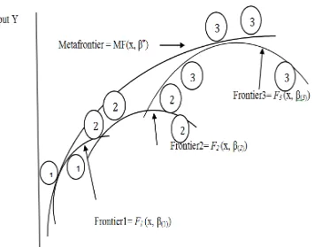
stochastic frontier functions for the different groups. A graph of the metafrontier function is presented

in Figure 1.

Three stochastic frontier models are indicated in Figure 1. The observed values are indicated by

numbers that corresponding (unobservable) stochastic frontier outputs are indicated by the numbers in circles above them. The values of the curves corresponding to the circled numbers can be considered as means of the potential stochastic frontier outputs for the given levels of the inputs. The metafrontier

function has values that are no less than the deterministic functions associated with the stochastic frontier models for the different groups involved. Some stochastic frontier outputs, and even their

corresponding stochastic frontier outputs, may exceed values of the metafrontier, as indicated in Figure 1.

The metafrontier model of equations (3) and (4) is related to the concept of the meta production function that was defined by Hayami and Ruttan (1971) as, “The meta production function can be regarded as the envelope of commonly conceived neoclassical production functions.” However, in our model, the metafrontier function is a production function of specified functional form that does not fall below the deterministic functions for the stochastic frontier

models of the groups involved. Battese and Ro (2002) give a more extensive literature review and proposed a stochastic metafrontier model that assumes a different data generation mechanism for the metafrontier than for the different group frontiers. The model in these papers assumes that

data-generation models are only defined for the frontier models for the farms in the different groups.

(4)

936 The observed output for the i-th farm at t-th time period, defined by the stochastic frontier for the j-th

group in equation (2), is alternatively expressed in terms of the metafrontier function of equation (3) by

(5)

where t-th first term on the right-hand side of equation (5) is the technical efficiency relative to the

stochastic frontier for the j-th group,

(6)

The second term on the right-hand side of equation (5) is the technology gap ratio (TGR) for the observation for the sample farm involved,

(7)

This measures the ratio of the output for the frontier production function for the j-th group relative to the potential output that is defined by the metafrontier function, given the observed inputs. The technology gap ratio has values between zero and one because of equation (4). The technical

efficiency of the i-th farm, given the t-th observation, relative to the metafrontier, denoted by TEit, is defined in an analogous way to equation (6). It is the ratio of the observed output relative to the last

term on the right-hand side of equation (5), which is the metafrontier output, adjusted for the corresponding random error, i.e.,

(8)

Equations (5)-(8) imply that n alternative expression for the technical efficiency relative to the metafrontier is given by

(9)

The technical efficiency relative to the metafrontier function is the production of the technical

efficiency relative to the stochastic frontier for the given group and the TGR. Because both the letter measures are between zero and one, the technical efficiency relative to the metafrontier is also between zero and one, but is less than the technical efficiency relative to the stochastic frontier

for the group of the farm. The parameters and measures associated with the metafrontier model of equations (2)-(4) can be estimated s follows:

Find the maximum-likelihood estimates ̂, for the β(j)-parameters of the stochastic frontier

for the j-th group using, for example, the FRONTIER program (Coelli, 1996);

Obtain estimates, ̂ , for the β*-parameters of the metafrontier function such that the estimated function best envelopes the deterministic components of the estimated stochastic frontiers for the different groups. To identify the best envelope, it is necessary to specify criterion that can be used

(5)

deviations and the other based on the sum of squares of deviations of the metafrontier values from

those of the group frontiers.

Estimates for the technical efficiencies of farms relative to the metafrontier function can be

predicted by

T ̂ ̂ ̂ (10)

where ̂ is the predictor for the technical efficiency relative to the given group frontier, as proposed in Battese and Coelli (1992); (Battese and Coelli, 1995), which is programmed to be calculated

in FRONTIER; and ̂ = ̂ is the estimate for the i-th farm in the j-th group relative to the industry potential, obtained by using the estimates for the parameters involved.

2.1. Minimum Sum of Absolute Deviations

Given the estimates for the parameters of the group stochastic frontiers ̂ , j = 1,2,……..,R, obtained by Step (1) above, the β*

-parameters can be estimated by solving the optimization problem below:

Min L ≡ ∑ ∑ | ̂ | (11) s.t. ̂ . (12)

There are several interesting features to the application of this criterion. First, the deviations used here are essentially logarithms of f(xit, β*)/ f(xit, ̂ ), which represent the radial distance

between the metafrontier and the j-th group frontier, evaluated t the observed input vector for farm in the j-th region. Thus the use of (11) and (12) implies that the resulting metafrontier minimizes the sum of logarithmic radial distances between the metafrontier and group frontiers.2 Second,

since the optimization is subject to the inequality restrictions in (12), all the deviations involved are positive and, therefore, the absolute deviations are simply equal to the deviations. Third, if f(xit, β*)

in equation (3) is assumed to be log-liner in the parameters (as it is in these papers), the optimization problem in (11) and (12) simplifies to the following linear programming (LP) problem:

Min L ≡ ∑ ∑ ̂ ) (13) s.t. ̂ (14)

The solution to the above problem is equivalently obtained by minimizing the objective function, β*, subject to the liner restrictions of (12), where is the row vector of means of

the elements of the xit-vectors for all observations in the data set. This follows because the estimates of the stochastic frontiers for the different groups, ̂ ,j = 1,2,……..,R, are assumed to be

fixed for the liner programming problem.

2.2. Minimum Sum of Squares of Deviations

Minimization of the objective function in (11) and (12) assigns the same weight for all the radial distances for all the farms in the sample. An alternative approach is to estimate the parameters of the

(6)

938 metafrontier function from the group- specific stochastic frontiers t the observed input levels. This

method assigns higher weights to the deviations associated with farms that have larger technology gap ratios. This leads to the following optimization problem:

Min L ≡ ∑ ∑ ̂ 2 (15) subject to the restrictions of equation (14).

This approach is similar to the use of the least-squares criterion. The optimization problem in (15), identical to constrained least-squares estimation, is quadratic programming (QP) problem that

minimizes the education distances of the values on the metafrontier from those on the estimated stochastic frontier functions. Standard errors for the estimators for the metafrontier parameters can

be obtained using simulation or bootstrapping methods.

3. EMPIRICAL APPLICATION

This paper uses data on farms in the Bangladeshi wheat farmers that were collected in the annual surveys of farms in the Bureau of Statistics for 2005-2010. Converge of these surveys in

basically restricted to medium and large scale establishments, which have at least 20 employees. Analyses of technical efficiency wheat farmers at the regional level are important and challenging for Bangladesh. From policy point of view, it is of interested to distinguish the regional differences

in mean efficiency levels and to determine whether the regions share some common characteristics. For the purpose of the present study, wheat farms are grouped into five regions: North, West,

Central, East and other region in Bangladesh (the other regions are pooled together because of the smaller numbers of farms in these regions). By performing the stochastic frontier analysis separately at the regional levels, the study permits the parameters of the empirical model to be different for these

five regions. The regional-levels analyses are believed to be desirable because it is likely that the wheat farms in the different regions are operating under different technologies. The estimation of the

metafrontier production function for the wheat farms enables a comparison of the technical efficiencies of farms in different regions, together with an analysis of the technology gaps of farms in particular regions, relative to the technology available to the farms as a whole.

Empirical results are obtained by using the stochastic frontier production model with time-varying inefficiency effects, proposed by Battese and Coelli (1992). The translog stochastic frontier

production function model, which is assumed to represent the production technology for wheat farms in particular region, is defined by

∑ ∑ ∑ (16)

where the Uits are assumed to be defined by

Uit = {exp[-η(t-T)]}Ui, i = 1,2, …., N; t = 1,2,…,6 (17)

In Yit denotes the natural logarithm of the total value of output for the i-th farm in the t-th year (in thousands taka’s, at 2005 constant prices);3 _x

1 denotes the natural logarithm of the total value of operating costs (including expenditures on electricity, fuel and lubricants, maintenance and repairs

(7)

of paid laborers, hereafter referred to as labor; x3 denotes the natural logarithm of the total value of

costs of raw materials purchased by the farm, hereafter called materials; x4 denotes the natural logarithm of the total amount of investments5(if positive) and zero otherwise (i.e., the logarithm of

the maximum of the investments and 1-D, where D denotes the dummy variable for the actual annual value of investments, which has value one if the farm had positive level of investments6 in the given year, and has value zero, otherwise); x5 denotes the time variable, where x5= 1, ….., 6 for 2005, ……,2010, respectively; (the subscripts, i and t, are omitted above for simplicity of presentation); the vits are assumed to be independently and identically distributed as N(0, σv2)

-random variables, independently of the Ui s

; the Ui s

are assumed to be independently and identically distributed non-negative random variables, obtained by truncation (at zero) of the (µ,σ2₎ -distribution; and the βs, η, σv2 and σ2 are unknown parameters to be estimated.

The stochastic frontier model, defined by equations (16) and (17), is estimated using data on wheat farms in a given region. The technical efficiency of the i-th farm, given the observation for

the i-th period, relative to its regional frontier, TEit = exp(-Uit), is predicted as proposed in Battese

and Coelli (1992). Thus the technical efficiencies of individual farms are generally estimated

relative to the technology of that region, as defined by the stochastic frontier model (16) and (17). However, the technical efficiencies of all wheat farms cross regions in Bangladesh can also be estimated relative to metafrontier function, as defined in section 2.

Basic summary of the observations on the variables for the different regions is presented in Table 1. These statistics indicted that there are considerable differences among the three regions so

far as the means and standard deviations of the outputs and inputs are concerned. The total number of farms involved in the five regions is 1,732 and the total number of observations for all farms is 6,385.

The maximum likelihood estimates of the parameters in the regional frontiers were obtained using the FRONTIER 4.1 program (Coelli, 1996). The null hypothesis that the technical

efficiencies effects were not present in given region, given the specifications of the stochastic frontier model, was rejected for all regions. Thus the technical inefficiencies were significant in all regions. The null hypothesis that the Cobb-Douglas frontier is an adequate representation of the

data was strongly rejected, as was the null hypothesis that there was no technical change8 in the wheat farms between 2005 and 2010, for all regions. It is important to examine if all the regions

share the same technology. If all the farm level data were generated from single production frontier and the same underlying technology, there would be no good reason for estimating the efficiency levels of farms relative to metafrontier production function. Likelihood-ratio (LR) test of the null

hypothesis that the regional stochastic frontier models are the same for all farms in Bangladesh was calculated after estimating the stochastic frontier by pooling the data from all the five regions. The

value of the LR statistic was 825.52,9 which are highly significant. This result strongly suggests that the five regional stochastic frontiers for farms in Bangladesh are not the same.

The preferred models for the technical inefficiency effects were not the same for the five regions. The

maximum-likelihood estimates for the parameters of the preferred stochastic frontiers production function for Bangladesh together with the estimates of the metafrontier obtained by linear and quadratic

(8)

940 variability of the metafrontier estimators, which derives from the sampling variability of the regional

frontiers estimates. Specifically, we used the estimated asymptotic distributions of the regional frontier estimators10 to draw M = 5,000 observations on the regional frontier parameters. Each draw was then used

to calculate the right-hand side of the constraints in new LP/QP problem. The estimated standard errors of the metafrontier estimators were calculated as the standard deviations of the M solutions to these LP/QP problems. All metafrontier results were obtained using the GAUSS programming language.

Table-1. Summary statistics for data on wheat farms in Bangladesh Variable North region West region Central

region

East region Other regions Output Mean St. Deviation 7,783,688 13,556,260 3,512,920 8,456,469 1,215,302 4,325,326 523,359 1,523,540 1,98,752 2,025,223 Capital Mean St. Deviation 66, 156 150,301 48,754 163,896 16,231 65,204 12,750 42,522 12,566 33,542 Labor Mean St. Deviation 358.20 672.40 243.36 370.45 206.35 286.31 100.49 205.32 101.32 160.22 Materials Mean St. Deviation 4,325,341 7,345,206 1,745,956 3,870,185 659,427 2,452,260 435,201 812,426 436,302 9,60,120 Investments Mean St. Deviation 3,568,425 32,785,450 6,025,586 47,820,541 2,258,654 24,752,452 457,025 14,98,425 1,265,026 20,283,524

Number of

farms

455 622 288 162 205

Number of obs. 1,805 2,345 1,025 650 560

Sources: Empirical results, based on Bangladesh BBS. (2005-2010). The values of output and inputs

expressed in thousands taka.

Table-2. Maximum likelihood estimates of the translog stochastic frontier for Bangladesh, together with estimates of parameters of the metafrontier production function.

Variable

Co-efficient

SF Met (LP) Meta (QP)

Constant β0 7.21(0.30) 8.33(0.38) 7.86(0.33)

Investments dummy β00 -0.2.15(0.088) 0.11(0.21) 0.03(0.19)

Capital β1 0.352(0.039) 0.563(0.083) 0.523(0.071)

Labor β2 0.975(0.054) 1.26(0.12) 1.19(0.11)

Materials β3 -0.576(0.029) -0.723(0.093) -0.705(0.08)

Investments β4 0.029(0.018) -0.048(0.045) -0.040(0.040)

Year β5 -0.032(0.028) 0.098(0.050) 0.076(0.042)

(Capital)2 β11 0.0125(0.0027) 0.021(0.0052) 0.0245(0.0049)

(Labor)2 β22 0.0455(0.008) 0.057(0.014) 0.059(0.013)

(Materials)2 β33 0.0832(0.0013) 0.108(0.0059) 0.104(0.0035) (Investments)2 β44 -0.00035(0.00061) 0.0025(0.0017) 0.0017(0.0016)

(Year)2 β55 0.0250(0.0015) 0.0284(0.0035) 0.0249(0.0035)

(9)

Labor × Materials β23 -0.1001(0.0052) -0.126(0.015) -0.116(0.012) Labor × Investments β24 -0.0002(0.0011) -0.0018(0.0025) -0.0028(0.0023) Labor × Year β25 0.0077(0.0041) 0.0162(0.0078) 0.0141(0.0072) Materials × Investments β34 0.00051(0.00062) 0.0021(0.0015) 0.0028(0.0013) Materials × Year β35 -0.0031(0.0027) -0.0226(0.0061) -0.0220(0.0056) Investments × Year β45 -0.00015(0.00045) -0.00031(0.00095) -.0011(0.0090)

Note: The estimated standard errors are given in parentheses correct to two-significant digits. The coefficient

estimates are given to the same number of digits behind the decimal points s standard errors

There are insignificant differences between the LP and QP estimates for the parameters of the metafrontier function, but there are significant differences between the metafrontier coefficients and

their corresponding coefficients of the stochastic frontier for Bangladesh. The latter estimates were used in Battese and Ro (2002) to approximate estimates for the parameters of the metafrontier function. These estimates gave unsatisfactory results for the technical efficiencies and the technology

gap ratios.

3.1. Technical Efficiencies and Technology Gap Ratios

Estimated values of the TGR, together with the technical efficiencies obtained from the regional stochastic frontier (TE) and metafrontier (TE*) were calculated for all farms in the different regions.

Basic summary statistics for these measures are presented in Table3, where the metafrontier technical efficiencies are from the LP estimates only (because those from the QP estimates were almost

identical to those from the LP estimates). The mean values of the technology gap ratio vary from bout 0.60 (for East region) to 0.90 (for north region). These results imply that, for East Bangladesh, the

wheat farms produce, on an average, only about 52% of the potential output given the technology available to the farms as a whole. However, farms in north region produce, on average, about 90% of the potential output. It is interesting to note that in all regions, except East Bangladesh, the regional

frontiers were tangent to the metafrontier (the maximum value for the technology gap ratio, namely one, was obtained each of these two regions). There was substantial variability in the technology gap

ratios for farms in all regions, but much less variability for farms in north region of Bangladesh

(BBS., 2005).

Wheat farms in Bangladesh achieved the highest mean technical efficiencies relative to the

metafrontier. For the other regions, the technical efficiencies calculated relative to the metafrontier function were substantially smaller than those calculated from the regional frontiers. Wheat farms

in East Bangladesh had the highest mean technical efficiency relative to their regional stochastic frontier, but they tended to be furthest from the potential outputs defined by the metafrontier function.

Table-3. Summary statistics for the TGRs and the technical efficiencies obtained from the regional stochastic frontiers and the metafrontier production function for Bangladesh wheat farms.

Region/Statistics Mean Minimum Maximum St. Dev.

North region Regional TE Tech. Gap Ratio Metafrontier TE*

0.890 0.903 0.632

.035 0.183 0.012

0.953 0.1.00 0.863

(10)

942

West region Regional TE Tech. Gap Ratio Metafrontier TE* 0.652 0.816 0.533 0.165 0.036 0.002 0.921 0.1.00 0.752 0.012 0.133 0.104 Central region Regional TE Tech. Gap Ratio Metafrontier TE* 0.712 0.602 0.431 0.363 0.226 0.103 0.976 0.1.00 0.796 0.019 0.093 0.084 East region Regional TE Tech. Gap Ratio Metafrontier TE* 0.822 0.602 0.436 0.361 0.406 0.104 0.936 0.820 0.723 0.089 0.092 0.084 South region Regional TE Tech. Gap Ratio Metafrontier TE* 0.761 0.632 0.311 0.353 0.121 0.074 0.932 0.100 0.825 0.122 0.154 0.133

Note: The linear programming estimates for the metafrontier co-efficient are used in this table

The study of the reasons for the wide variations in the TGRs and the technical efficiencies in the different regions for both the regional stochastic frontiers and the metafrontier is worthy of further

investigation.

4. CONCLUSIONS

The main objective of providing comparable technical efficiency score for farms across different technologies, metafrontier production function model is proposed and applied in the analysis of the

technical efficiencies of wheat farms in five regions in Bangladesh. The methodology proposed enables the estimation of regional TGRs by using a decomposition result involving both the

regional stochastic frontiers and the metafrontier. Further theoretical and applied studies with other models for technical inefficiency effects are clearly desirable.

Notes

1. For a translog production function, xit(j)would contain the logarithm of the different inputs,

their squares and cross-products

2. The radial distance is used in defining the input and output distance function that forms the basis for all productivity comparisons. Coelli et al. (1998), Chapter 3.

3. All variables that are in monetary units are in thousands of taka, expressed in 2005 prices. 4. The total operating cost is used as proxy for the value of capital services.

5. Investments are specified in the production function because they are usually targeted at the upgrading of technology and so they could be associated with technological changes.

6. Because investments were not always positive, the dummy variable, D, is used for handling

zero observations, as proposed by Battese (1997).

7. The subscript, used in equations (1)-(15) to distinguish particular region, is not include in the

empirical model of equation (16) for simplicity of presentation.

8. This refers to no time effects (or exogenous technological changes) in the production frontier. However, as stated in the specification of the frontier model in equation (16), the level of

(11)

technical change involves testing that all coefficients associated with time and investments

were zero.

9. The LR statistic is defined by λ=-2{ln [L(H0)/ L(H1)]} = - 2{ln [L(H0)] –ln[ L(H1)]}, where

ln[L(H0)] is the value of log-likelihood function for the stochastic frontier estimating by pooling the data for all regions and ln[ L(H1)] is the sum of the values of the log-likelihood functions for the five regional production frontiers. The degrees of freedom for the chi-squares

distribution involved are 104, the difference between the numbers of parameters estimated under H1 and H0.

10. The parameters of the regional frontiers were estimated by maximum likelihood so the estimators are asymptotically normally distributed.

A Metafrontier Production Function for Estimation of Technical Efficiencies of Wheat Farmers under Different Technologies