Characterisation and modelling of structural bonding at high strain rate

c

Owned by the authors, published by EDP Sciences, 2012

Characterisation and modelling of structural bonding at high strain rate

G. Haugou

_{, B. Bourel}

_{, F. Lauro}

_{, B. Bennani}

_{, D. Lesueur}

_{, and D. Morin}

1_{Univ. Lille Nord de France, 59000 Lille, France}

2_{UVHC, LAMIH, UMR CNRS FRE 8201, 59313 Valenciennes, France}

3_{Norwegian University of Science and Technology, SIMLab, N-7491 Trondheim, Norway}

Abstract. These paper deals with the development of new bonded joint modelling for crash application. A new testing device has been set up on Split Hopkinson bars in order to identify adhesive’s properties in assemblies for high strain rate and for different loading angles. These tests led to the development of a new cohesive element model used for solving nonlinear dynamic problems with an explicit integration time scheme. An example illustrates and justifies the development of such a cohesive element under dynamic loading by a good efficiency and a significant saving in calculation time.

1 Introduction

The structural bonding is an assembling technique that has recently gained much interest in the industry and partic-ularly in automotive. It provides many advantages, espe-cially with the aim of lightening structures. It allows more particularly to join different materials (steel, aluminium, polymers) and also to reduce the stress concentrations compared to spot welding. But to be validated for its use in crash applications, structural bonding needs to be tested extensively for a wide range of strain rate.

In the literature, two kind of test are used to charac-terize the behaviour and the failure of the bonded joints. The first are achieved on bulk adhesive specimens [1, 2]. Yet little used, these tests have the advantages to obtain a very homogeneous stress state inside the specimens. The second technique, mainly used, is performed by achieving test directly on assemblies. Tensile/compressive, shear and mixed loadings are obtained with butt, single or double lap and scarf joints respectively [3–5]. The benefit of these tests is the characterization of bonded joints in conditions near those used in industry. The problem is that these experiments are only conducted at low strain rate not exceeding the 500 s−1.

From a numerical point of view the mechanical prop-erties of the adhesive suffer of a lack of models in the lit-erature. A fine description of the adhesive properties, with a visco-plasticity behaviour based on a bilinear Drucker-Prager yield criterion and with a failure model based on an equivalent failure strain evolving with the strain rate and the triaxiality stress ratio was recently developed in [6, 7]. But, the main limitation of such a modelling in the industrial context come from its small time step leading to a very expensive Finite Element calculation time with the explicit integration scheme. To avoid this problem some special purpose cohesive element based on a spring element formulation, have been developed.

The proposed works are then composed by an exper-imental part and a numerical part. Experexper-imentally, a new testing device is developed to analyse the mixed stress effect on the behaviour and the failure of bonded joints at high strain rates. This work supplements previous work done with strain rates up to 500 s−1_{. Cylindrical bonded}

assemblies are designed and tested on a set of the split Hopkinson tensile bars device to obtain the glue charac-terization at high strain rate. Different loading angles are tested to study the effect of mixed constraints on such as-semblies. On the numerical aspect, these experiments have enriched the cohesive element developed in [8], especially by including an equivalent spring formulation instead of three independent springs, by using a real yield surface, and also by improving the representativeness of the model at very high strain rate. These developments have been tested and successfully validated on some examples of structures subjected to dynamic loadings.

2 Experimental testing

In the field of crashworthiness of transportation structure, experiments need to be as representative as possible, and must cover a wide range of loading conditions such as angle and strain rates. Many tests have previously been done on bulk adhesive as well as on assemblies [2, 9]. However, data are missing for tensile and shear loadings at high strain rates.

As mechanical responses of bonded joints depend on the loading angle coupled with velocity effect, Hopkin-son bars technique is proposed in their tensile version (figure 1). Here, cylindrical bars made of high strength steel with 30 mm in diameter are used, and loaded by means of a tubular striker made of aluminium (1 m in length). The overall length of the device is close to 10 m.

Special connectors are developed to test bonded assem-blies on measurement bars. Three configurations are done with different loadings angles: pure tension (0◦), shear (90◦), and mixed-mode loadings (45◦). The preparation process is described below:

– The cartridge of glue is pre heated at 60◦C, the connec-tors are aligned in a special mounting.

– The glue is deposited at the free surface of the con-nectors and its thickness is calibrated with glass ball (300µm),

– All connectors are cured at 170◦C during 45 min and finally refreshed to room temperature with a slope of 15◦C/min.

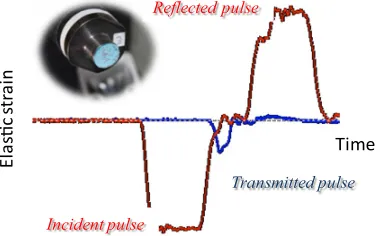
Incident pulse

Transmitted pulse

Fig. 2.Typical raw data signal – Tensile loading at 0◦.

Fig. 3.Bonded joint assemblies at 0◦, 45◦and 90◦.

Typical signals recorded during the tests are presented in figure 2 and detected by full strain bridges cemented at strategic locations along the bars so as to avoid any reflection of the elastic waves’ system The data acquisition is ensured using a digital oscilloscope at a sampling rate of 10 Ms/s to capture precisely both elastic and non linear domains of the bonded joints.

In the present study, the elongation at break is par-ticularly short so that classical analysis of the elastic waves’ system cannot be done. Therefore, the current elongation of the joint is measured using an electro-optical extensometer (Rudolph XR200 – measuring range: 5 mm – resolution: 5µm). This equipment gives the opportunity to access to very high accuracy coupled with high bandwidth.

The specimen elongationδ(t) is given by:

δ(t)=δIB(t)−δOB(t) (1) where,δIB(t) andδOB(t) are respectively, the displacement of the input and output bars. Whatever, the calculation of the force transmitted through the sample FOB(t) is still performed using the governing mentioned in the literature: FOB(t)=SOB×EOB×εT RA(t) (2) where SOB and EOB are respectively the section and the elastic modulus of the output bar.εT RA(t) is the transmitted elastic signal in function of time.

As the initial thickness is close to 0.3 mm (figure 3), the strain rate level has increased over 9000 s−1.

In figure 4 are related the typical responses force/ displacement of the bonded joint according to the three loading angles mentioned previously.

In pure tension, adhesive’s behaviour appears to be al-most elastic-brittle, with very small plastic zone. Indeed, it

0

0 0.1 0.2 0.3 0.4 0.5 0.6

Displacement (mm)

Fig. 4.Synthesis of the structural bonding responses at 0, 45 and 90◦with the SHTB device.

Fig. 5.Representation of the cohesive element.

can be seen on the failed samples a slight whitening of the adhesive. This is also true for the mixed tensile/shear tests. The shear tests show a higher response of the adhesive joint with a distinct plastic zone.

The mixed tensile/shear seem nevertheless wrong since an intermediate behaviour between the pure tension and pure shear was expected. This may be due to the small amplitude of the transmitted signal. It could be corrected by increasing the cross section of the sample.

3 Bonded joint modelling

The present results are then exploited to model the adhe-sive behaviour. A coheadhe-sive element approach is used. At the boundary between the CCZM (Continuous Cohesive Zone Method) and the DCZM (Discrete Cohesive Zone Method) approaches, the proposed cohesive element in-cludes an improved constitutive model in order to take into account the viscoplasticity of the adhesive, its different behaviour in tension and compression but also its damage and failure cracks propagation.

3.1 New cohesive element description

The cohesive element developed has a non-zero volume imposed by the thickness of the adhesive layer. This element, based on a 8-node hexahedron element, can however be seen as a generalized spring between the two structural elements opposite each other (figure 5). This discrete spring is attached to the centres of the lower face

Γ−_{and the upper faceΓ}+_.

Fig. 6.Original simplified behaviour law of the adhesive.

of both. The main advantage of such a modelling comes from the generalized spring time step. Contrary to classical solid element, the spring time step does not depend on the element size. It only depends on the spring stiffnesskand the massesm1andm2assigned to the lower and upper face:

∆tcrit=2

m1m2 m1+m2

.1

k (3)

m1andm2correspond to the structural element masses on

both sides of the joint, increased by half of the adhesive mass contained in the volume of the cohesive element.

3.2 Constitutive law

This cohesive element includes an improved constitutive model in order to take into account the viscoplaticity of the adhesive, its different behaviour in tension and compression but also its damage and failure (figure 6).

3.2.1 Elasto-viscoplasticity

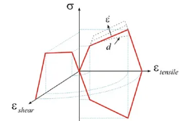
The elastic modulus and yield stress identification is per-formed in tension for 5 strain rates ranging from 50 s−1to 13300 s−1. Even if the material has strain rate sensitivity, this sensitivity can be neglected for the elastic part in ap-plications such as crash. Consequently, the elastic modulus is assumed to be insensitive to the strain rate. An equivalent yield criterion has been proposed. The yield surface shown on figure 7 is given by:

fn=σ¯ −ασ_y=0 (4)

where αy is the yield stress in tension and ¯σ is the equivalent stress given:

¯

σ= (ασn)2_+σ2

t (5)

σn andσt are respectively the normal and the tangential stresses in the element. The parameterαis used to repre-sent the yield difference between tension/compression and shear. This parameter is obtained from the assemblies tests described in section 2.

The yield stress evolution versus the strain rate is expressed by a Johnson-Cook law:

σy=σy0

1+blog ε˙¯ ˙ ε0

(6)

Fig. 7.Yield surface of the cohesive element.

whereσy0,band ˙ε0are material parameters identified

ex-perimentally. Finally, the strain rate effect on the structural hardening is performed by viscous tangent modulus. Its evolution follows the polynomial model expressed by:

ET=c0+c1ε˙¯+c2ε˙¯2+c3ε˙¯3 (7)

whereσ_y0,band ˙ε0are constant parameters obtained with

tensile tests.

3.2.2 Damage

The damage evolution is obtained by measuring the vol-ume variation in the adhesive material during tensile tests using Digital Image Correlation measurements. In the proposed model, this evolution is based on the longitudinal strainεnassuming compressive and shearing strains do not contribute to void growth:

d=d0+d1

1−ed2(ε0−εn) ₍₈₎ d0,d1andd2are constant parameters obtained with tensile

test.

3.2.3 Failure

The failure of the cohesive element is based on a crack initiation criterion and on a crack propagation through the element length. The initiation criterion depends on the openingδnand sliding displacementδtbetween the lower and upper element faces. Assuming that the compression has no influence on the crack propagation, it can be written as follows:

λ= δt1 δcrit t1

2

+δt2 δcrit

t2

2

>1 if δn>0 (9)

λ=

δn δcrit

n

2

+δt1 δcrit

t1

2

+δt2 δcrit

t2

2

>1 if δn <0 (10) The dynamic tests on assemblies have shown a strong dependency of the failure strain to strain rate. A model for opening and sliding critical displacements is then identified:

δcrit _ε˙¯=δ

0

1+nlog ε˙¯ ˙ ε0

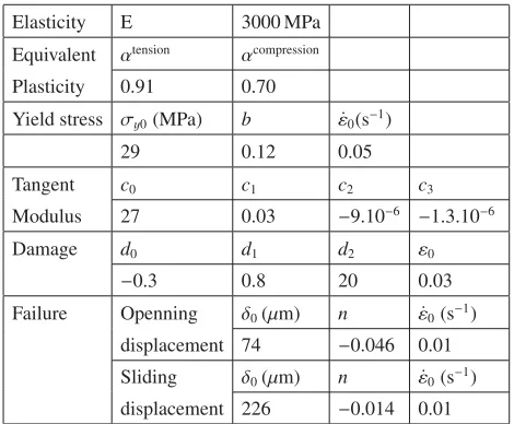
Tangent c0 c1 c2 c3

Modulus 27 0.03 −9.10−6 _−1.3.10−6

Damage d0 d1 d2 ε0

−0.3 0.8 20 0.03

Failure Openning δ0(µm) n ε˙0(s−1)

displacement 74 −0.046 0.01

Sliding δ0(µm) n ε˙0(s−1)

displacement 226 −0.014 0.01

to define a crack propagation speed. In our model, this propagation speed is assumed to be proportional to the equivalent opening speed.

Vp=κ·Veq with Veq=

˙ δ2

n +δ˙2t1 +δ˙2t2 (12)

All material parameters required for this cohesive element model are given in Table 1.

4 Numerical implementation

The proposed cohesive element is implemented in the nonlinear dynamic explicit software ABAQUS through a VUEL subroutine. This implementation occurs in the time loop for the internal forces calculation. A special analysis is then applied to each cohesive element used in the FE model.

4.1 Strain and strain rate computations

After construction of the local element basis (n,t1,t2), the

relative displacement vector between the upper and the lower face of the element is written:

δ=u(Γ+)−u Γ−R (13) whereu(Γ+) andu(Γ−) are the displacement at the centre of the element upper and lower faces. R denotes the transfer matrix from the global basis to the local basis. The strain state at the centre of the element can then be calculated by:

εn=ln1+ _Lδn n,0

(14) εt=arctan1+ _Lδt

n,0

(15) where δn_, δt respectively denotes the opening (following the normal direction n) and the sliding (following the transversal direction t) displacement. Ln,0 is the initial

thickness of the cohesive element.

After an elastic prediction, an equivalent stress is com-puted from (5). If ¯σ ≤ ασ_y there is no plastic strain and the stresses are not corrected. If ¯σ > ασ_y, the elastic limit is reached and a yield return must be calculated. In this second case, an equivalent plastic strain εp is calculated and the equivalent stress is updated according to:

¯

σ=σy+(1−d)ETεp¯ with εp¯ =∆_Eσ¯ (17)

where the tangent modulus ET _{and the damage variable} d are respectively calculated from eq.(7) and eq.(8). After updating the equivalent stress, a first projection is made in the plane (σn, σt). The components σn and σt are computed by using the loading angle defined by θ = arctan(εn/εt):

σn= σ_α¯ sin(θ) and σt=σ¯cos(θ) (18)

Then a projection ofσtis made in the plane (σt1,σt2):

σt1 =σtsin(β) and σt2 =σtsin(β) (19)

whereβis the angle defined byβ=arctan(εt1/εt2).

The internal forces calculated at the nodes of the cohesive element in the global basis (x,y,z) are then given by:

Fnx=F n−1

x +(∆σnn+∆σt1t1+∆σt2t2)·x·S0(1−d)

(20) F_yn=Fn_y−1+(∆σnn+∆σt1t1+∆σt2t2)·y·S0(1−d)

(21) Fzn=F

n−1

z +(∆σnn+∆σt1t1+∆σt2t2)·z ·S0(1−d)

(22) withS0the initial cross section of the element andσn,σt1

andσt2the stress increments expressed in the local basis.

4.3 Element failure

After detection of the crack initiation eqs. (9-10), the element is progressively eliminated. Numerically, too fast elimination would lead to elastic wave release which would bring numerical instabilities. So, the element elimi-nation is carried out by introducing the crack propagation speedVpdefined by eq.(12). Consequently, that determines the time trup_{at which the element is completely removed} from the simulation:

trup= Lx,0 Vp

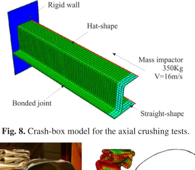
Fig. 8.Crash-box model for the axial crushing tests.

Fig. 9.Experimental (a) and numerical (b) deformed shape.

whereLx_,0 is the element length in the crack propagation

direction. This leads to a new stresses update (at timetn₎ for the element elimination phase:

σn₌ σinit trup

tinit−tn+σinit ₍₂₄₎ where tinit _{and σ}init _{are respectively the time and the} stress at the failure initiation. During the elimination phase, the internal forces are obtained with the same relations (eq. 20–22) from the new updated stress.

5 Validation

The proposed element is tested on bonded thin-walled closed-hat section profiles subject to an axial crushing impact.

5.1 Test case description

In a first study, a single bonded joint configuration (without spot-welds) and an adhesive thickness of 0.3 mm between the hat-shape and the straight-shape is considered. This crash-box is impacted by a mass of 350 kg with a velocity of 16 m/s (figure 8). The steel grade used in this example is a DP600 with a thickness of 1.5 mm. The steel behaviour is modelled using a viscoplastic model through the input of tabulated true strain/true stress curves.

5.2 Experimental/numerical comparison

The numerical results have been compared to experimental tests. A good agreement between the two approaches is observed in terms of deformed shapes (figure 9).

Experimentally, the buckling of the steel plates is observed. Due to the adhesive failure the straight-shape of the crash-box opens during folding. However a reasonable energy dissipation value is obtained in such a configuration (around 9 kJ).

Fig. 10.Dissipated energy curves.

Table 2.Computation time comparison.

With With classic With classic cohesive solid elements solid elements (1 element) (3 elements) (3 elements)

CPU Time 4 min 16s 211 min 11s 4600 min 00s

The finite element analysis carried out with the pro-posed cohesive element is able to predict the section open-ing as observed experimentally. Otherwise, the figure 10 shows the dissipated energy during the crushing of the closed-hat section. According to this figure, experiments are performed on 5 specimens. Even if the numerical result seems to over-value this energy at the beginning of the deformation, it remains very close to the mean curve.

5.3 Calculation time saving

In order to study the benefit of our cohesive element on the calculation time, a similar simulation is performed with a bonded joint modelled with classic solid elements. In this model, the adhesive behaviour is implemented as a VUMAT subroutine in the ABAQUS software. It includes a viscoplastic behaviour based on an accurate bilinear Drucker-Prager yield criterion and an advanced failure model based on a critical equivalent failure strain.

Two calculations are performed with this VUMAT: one calculation with 1 element in the thickness of the adhesive joint and one calculation with 3 elements in the thickness. The obtained results in terms of energy dissipation are shown in figure 10. With this new accurate modelling, the use of 1 element in the thickness of the joint seems to be sufficient. But, even with this modelling, the dissipated energy is very close to those obtained with the proposed cohesive element.

But the drawback with this approach is the very small element time-step leading to an expensive calculation time. A summary of the computation times for the three Finite Element models used is proposed in table 2. The accurate modelling leads to a big increase in the computational time (greater than 1000% for only one element in the thickness).

6 Conclusions

modelling compared to a more accurate model. When the improvement on the global response is balanced with the computation time, the choice of a macroscopic modelling is therefore fully justified.

Consequently, even if today there are different ways to model adhesive joints, this macroscopic approach seems to be the best suited to industrial needs, mainly thanks to its simplicity for calibration when compared to the existing cohesive element, its simplicity of implementation, and its interest in terms of computation time.

Acknowledgements

The present research work has been supported by CISIT, the International Campus on Safety and Intermodality in Transporta-tion, the Nord-Pas-de-Calais Region, the European Community, the Regional Delegation for Research and Technology, the Min-istry of Higher Education and Research, and the National Center for Scientific Research. The authors gratefully acknowledge the support of these institutions.

References

1. L. Goglio, L. Peroni, M. Peroni, M. Rossetto, High strain-rate compressive and tension behaviour of an epoxy bi-component adhesive. International Journal of Adhesion and Adhesives, 28 (2008), 329–339.

extension rates and temperatures. International journal of adhesion and adhesives, 23 (2007), 1–15.

4. M. You, Z.M. Yan, X.L. Zheng, H.Z. Yu, Z. Li. A numerical and experimental study of gap length on adhesively bonded aluminium double-lap joint. International Journal of Adhesion and Adhesives, 27 (2007), 696–702.

5. G. Dean, L. Crocker, B. Read, L. Wright. Prediction of deformation and failure of rubber-toughened adhesive joints. International Journal of Adhesion and Adhe-sives, 24 (2004), 295–306.

6. D. Morin, G. Haugou, B. Bennani, F. Lauro. Exper-imental characterization of a toughened epoxy adhe-sive under a large range of strain rates. Journal of Adhesion Science and Technology, 25 (2011), 1581– 1602.

7. F. Lauro, B. Bennani, D. Morin, A. Epee. The SEE method for determination of behavior laws for strain rate dependent material: application to polymer mate-rial. International Journal of Impact Engineering, 37 (2010) 715–722.

8. D. Morin, B. Bourel, B. Bennani, F. Lauro, D. Lesueur. A new cohesive element for structural bond-ing modellbond-ing under dynamic loadbond-ing. International Journal of Impact Engineering, Special Issue ICILLS (2012) – Accepted.