A Step toward Decision making in Diagnostic
Applications using Single Agent Learning
Algorithms
Deepak A. Vidhate
1, Dr. Parag Kulkarni
2 1Research Scholar College of Engineering Pune
2EKLaT Research Pune
Abstract –
The output of the system is a sequence of actions in some applications. There is no such measure as the best action in any in-between state; an action is excellent if it is part of a good policy. A single action is not important; the policy is important that is the sequence of correct actions to reach the goal. To be able to generate a policy the machine learning programs should able to assess the quality of policies and learn from past good action sequences.
Learning is the basic capacity of intelligent agents. An agent changes its behavior based on its previous experiences through learning. An intelligent agent must be formalized by knowledge and be able to act on this knowledge. In many single-agent systems for learning the policy of an agent in uncertain environments, the reinforcement learning techniques have been applied successfully. Many existing single-agent models for sequential decision making are derived from a general model and are distinguished by assumptions. Q-learning algorithms are used for this purpose.
Single agent learning model is given in this paper. Four single agent reinforcement learning algorithms are implemented and results are compared. Single agent Q-learning Algorithm and Sarsa Learning Algorithm gives some results for the problem. However adding eligibility traces in single agent learning algorithms i.e. Q(λ) learning and Sarsa(λ) learning gives performs better than the previous algorithms. The paper shows the results of all four algorithms and performance comparisons among them.
Keywords – Q-learning, Reinforcement learning, Sarsa Learning, Single Agent
I. INTRODUCTION
Consider the example market chain that has hundreds of stores all over a country selling thousands of goods to millions of customers. The point of sale terminals record the details of each transaction i.e. date, customer identification code, goods bought and their amount, total money spent and so forth. This typically generates gigabytes of data every day. What the market chain wants is to be able to predict who are the likely customers for a product. Again, the algorithm for this is not evident; it changes over time and by geographic location. If stored data is analyzed and turned into information then it
becomes useful so that we can make use of an example to make predictions[1].
We do not know exactly which people are likely to buy this product, or another product. We would not need any analysis of the data if we know it already. But because we do not know, we can only collect data and hope to extract the answers to questions from data.
We do believe that there is a process that explains the data we observe. Though we do not know the details of the process underlying the generation of data – for example, customer behavior - we know that it is not completely random. People do not go to markets and buy things at random.
When they buy beer, they buy chips; they buy ice cream in summer and spices for Wine in winter. There are certain patterns in the data. We may not be able to recognize the process completely, but still we can construct a good and useful approximation. That approximation may not explain everything, but may still be able to account for some part of the data. Though identifying the complete process may not be possible, but still patterns or regularities can be detected. Such patterns may help us to understand the process, or make predictions. Assuming that the near future will not be much different from the past and future predictions can also be expected to be right.
independent tasks that can be handled by separate agents could benefit from cooperative nature of agents[2].
Another example of a domain that requires cooperative learning is hospital scheduling. It requires different agents to represent the regard of different people within the hospital. Hospital employees have a different outlook. X-ray operators may want to maximize the throughput on their machines. Nurses in the hospital may want to minimize the patient’s time in the hospital. Since different people examine candidate with different criteria, they must be represented by cooperative agents. The output of the system is a sequence of actions in some applications. There is no such measure as the best action in any in-between state; an action is excellent if it is part of a good policy[3]. A single action is not important; the policy is important that is the sequence of correct actions to reach the goal. To be able to generate a policy the machine learning programs should able to assess the quality of policies and learn from past good action sequences[4]. This paper is organized as Section II gives the concept of single agent learning, Section III describes Q-learning algorithm, Sarsa learning algorithm is given in Section IV. Section V gives the description about eligibility traces to be added in learning algorithm and Section VI gives experimental setup. Section VII put up the result comparisons of all four algorithms and finally concluding remark with the future scope.
II. SINGLE AGENT LEARNING
Learning is the basic capacity of intelligent agents. An agent changes its behavior based on its previous experiences through learning. An intelligent agent must be formalized by knowledge and be able to act on this knowledge. In many single-agent systems for learning the policy of an agent in uncertain environments, the reinforcement learning techniques have been applied successfully[5].
It is possible to treat a multiagent system as a `large’ single agent to learn the optimal joint policy using standard single-agent reinforcement learning methods. However, both the state and action space size exponentially with the number of agents. Representation this approach is infeasible for most problems. Reinforcement learning techniques are mainly helpful in the field where reinforcement information (expressed as penalties or rewards) is supply after a series of actions carried out in the environment[6]. Q-Learning, Sarsa and Temporal-Difference (TD) Learning are common RL methods.
Single Agent Model
Many existing single-agent models for sequential decision making are derived from a general model and are distinguished by assumptions about the parameters of the general model. An overview of the relevant model parameters for single agent systems are given here and some related issues are discussed[7]. A discrete environment is focused for simplicity which has a finite number of states and actions.
Parameters
A finite, discrete sequential decision-making problem can be specified using the following model parameters:
A discrete time step t = 0, 1, 2, 3, . . . .
A finite set of environment states S. A state st є S
describes the state of the system at time step t.
A finite set of actions A. The action selected at time step t is denoted by atє A.
A reward function R: S × A → R which provides the agent with a reward rt+1 = R(st, at) based on the action at
taken in state st.
A state transition function T: S×A×S → [0, 1] which gives the transition probability p(st|at−1, st−1) that the
system moves to state st when the action at−1 is performed
in state st−1.
Markov Decision Process
Markov Decision Processes (MDPs) are the mathematical foundation for Reinforcement Learning in a single agent environment.
Definition 1: Markov Decision Process is defined by (S, A,T, R). S is a finite discrete set of possible states. A is a finite discrete set of possible actions. T is an unknown transition function giving for each state and action T: S×A→S. R is an unknown real-valued reward function of the agent R: S×A→R.
Solution techniques
To compute an optimal policy π* for a given MDP is given. An optimal policy should for every possible situation return the action that maximizes the performance measure. The solution is found out by two techniques i.e. model based and model free techniques. Model-based techniques require a complete description of the model, while model-free techniques, also referred to as reinforcement learning, only learn based on the received observations and rewards.
III. Q-LEARNING ALGORITHM
The problem is modeled using a Markov decision process (MDP). The rewards and the result of actions are not deterministic so it has a probability distribution for the reward p(rt+1|st,at) from which rewards are sampled and there is a
probability distribution for the next state P(st+1|st,at). These
help to model the uncertainty in the system that may be due to forces we cannot control in the environment. The Q-learning algorithm is used for this purpose[8].
reinforcement signal r є R that is then used to evaluate the quality of the decision by updating the corresponding Q(s, a) values[9].
The policy π defines the agent’s behavior and is a mapping from the states of the environment to actions. π : sa . The policy defines the action to be taken in any state. The value of a policy π, Vπ(s
t) is the expected cumulative reward that will
be received while the agent follows the policy, starting from state st.
Algorithm : Q Learning
1. initialize all Q(s, a) to 0 arbitrarily 2. for all episodes
3. initialize s 4. repeat
5. choose a using policy derived from Q e.g.
-greedy policy6. take action a, observe r and s’ 7. update Q(s, a) as
8. Q(s, a) Q(s, a) +α (r + γ maxa Q(s’, a’) – Q(s, a))
9. ss’
10. until s is terminal state
Discount rate parameter0 ≤γ< 1. It is considered as γ= 0.9. If γ =0, then only the immediate reward counts. As γ
approaches 1, rewards further in the future count more, and it is said that agent becomes more farsighted. γ is less than 1 because there generally is a time limit to the sequence of actions needed to solve the task. The value of learning rate parameter α is gradually decreased in time for convergence and it has been shown that this algorithm converges to the optimal Q values.
Steps in Q-Learning algorithm:
Below steps are followed as actual implementation of learning update rule involved in Q-learning for continuous time MDP. Let t0=0 and start with an initial arbitrary guess Q(s, a) = 0.
Step 1: At any nth transition epoch at time t
n, observe the state
s and select the product action a є argmaxa Q(s, a)
with probability 1-ε and other product in A with probability ε for some ε>0.
Step 2: If X(tn)=s and the product action was chosen is a then
update its Q value as follows:
Q(s, a) Q(s, a) +α (r + γ maxa Q(s’, a’) – Q(s, a))…..(1) To explore, one possibility is to use
-greedy policy search where with probability
we choose one action uniformly randomly among all possible actions i.e. explore and with probability 1 -
, we choose the best action i.e. exploit. We do not want to continue exploring indefinitely but start exploiting once we do enough exploration. For this, we start with a high
value and gradually decrease it.Repeat steps 1 & 2 infinitely. Convergence is slow as it is typical RL algorithm. The speed of convergence can be drastically improved using function approximations to Q-values based on some observed features.
Initially all Q(s, a) are 0 and they are updated in time as a result of trial episodes. Let us say we have a sequence of moves and at each move, we use above equation to update the estimate of Q-value of the previous state-action pair using the Q-value the current state-action pair. In the intermediate states, all rewards and therefore values are 0, so no update is done. When we get to the goal state, we get the reward r and then we can update the Q-value of the previous state-action pairs as γr.
IV. SARSA LEARNING ALGORITHM
Sarsa is an on policy version of Q-learning where policy is used to determine also the next action. Instead of looking for all possible next actions and choosing the best, the on policy Sarsa uses the policy derived from Q-values to choose one next action a and uses its Q-value to calculate the temporal difference. On policy methods estimate the value of a policy while using it to take actions. They approximate Q-value, the action values for current policy, and then improve the policy gradually based on the approximate values for the current policy[10]. The policy improvement can be done in the simplest way using ε-greedy policy with respect to current action value estimation. Sarsa learning algorithm is used for this purpose.
Algorithm : Sarsa Learning
1. initialize all Q(s, a) to 0 arbitrarily 2. for all episodes
3. initialize s 4. repeat
5. choose a using policy derived from Q e.g.
-greedy policy6. take action a, observe r and s’ 7. update Q(s, a) as
8. Q(s, a) Q(s, a) +α (r + γ Q(s’, a’) – Q(s, a)) 9. ss’ aa’
10. until s is terminal state
V. ELIGIBILITY TRACES
Q(λ) Learning Algorithm
Q-learning is an off policy method, meaning that the policy learned about need not be the same as the one used to select actions. Mainly Q-learning learns about the greedy policy. Typically Q-learning follows a policy involving exploratory actions. Special concern is required when introducing eligibility traces because of this[12]. Q(λ) does not look ahead all the way to the end of the episode in its backup. It only looks ahead as far as the next exploratory action. Watkins’s Q(λ) looks one action past the first exploration using its knowledge of the action values. Eligibility traces are manipulated just as in Sarsa(λ)[13]. They are set to zero whenever an exploratory (non-greedy) action is taken.
Model for Eligibility traces:
The trace update is thought of as occurring in two steps. First, the traces for all state-action pairs are either decomposed by
γλor if an exploratory action was taken, set to 0. Second, the trace corresponding to the current state and action is incremented by 1. The overall result is et(s, a) =
ম
sst.ম
aat + γλet-1(s, a) if Qt-1(st, at) = maxaQt-1(st, at)= 0 otherwise
whereas before
ম
xy is an identity indicator function, equal to 1if x = y and 0 otherwise. The rest of the algorithm is defined by
Qt+1(s, a) = Qt(s, a) + αδtet(s, a)… ……….(2)
where
δt = rt+1 + γmaxaQt(st+1, a’) – Qt(st, at)
Cutting off traces every time an exploratory action is taken loses much of the advantages of using eligibility traces.
Algorithm : Q(λ) algorithm
1. initialize Q(s, a) arbitrarily and e(s, a) = 0 for all s, a 2. repeat for each episode
3. initialize s, a
4. repeat for each step of episode 5. take action a, observe r, s’
6. choose a’ from s’ using policy derived from Q (ε -greedy)
7. a* argmaxb Q(s’, b) 8. δ r + γQ(s’, a*) – Q(s, a) 9. e(s, a) e(s, a) + 1 10. for all s, a
11. Q(s, a) Q(s, a) + αδe(s, a)
12. If a’ = a* then e(s, a) γλe(s, a) else e(s, a) 0
13. s s’; a a’ 14. until s is terminal
Sarsa(λ) Learning Algorithm
The eligibility trace version of Sarsa is called as Sarsa(λ). The scheme in Sarsa(λ) is to relate the TD(λ) prediction method to
state-action pairs rather than to states. Let et(s, a) denote the
trace for state action pair s, a; substituting state action variables for state variables the equation becomes
Qt+1 = Qt(s,a) + αδtet(s, a) for all s, a………..(3)
where
δt = rt+1 + γQt(st+1, at+1) – Qt(st, at)
and
et(s, a) = γλet-1(s, a) + 1 if s=st and a=at
= γλet-1(s, a) otherwise
One step Sarsa and Sarsa(λ) are on policy algorithms. The one step method strengthens only the last action of the sequence of actions that led to the high reward, whereas the trace method strengths many actions of the sequence. The degree of strengthening falls off (according to γλ) with steps from the reward[14].
Algorithm : Sarsa (λ) algorithm
1. initialize Q(s, a) arbitrarily and e(s, a) = 0 for all s, a 2. repeat for each episode
3. initialize s, a,
4. repeat for each step of episode 5. take action a, observe r, s’
6. choose a’ from s’ using policy derived from Q (e.g. ε greedy)
7. δ r + γQ(s’, a’) – Q(s, a) 8. e(s, a) e(s, a) + 1 9. for all s, a
10. Q(s, a) Q(s, a) + αδe(s, a) 11. E(s, a)γλe(s, a)
12. s s’; aa’ 13. until s is terminal
VI. EXPERIMENTAL SETUP
Model design:
Maximize the sale of products that depends on price of product, customer age and period of sale. These are the information available to each agent i.e. shop. So it becomes the state of environment. Final result is to maximize profit by increasing total sale of products.
Input Data set:
We define the action set as the sale of possible product. i.e. A={p1,p2,p3…….p10}
Hence action a
A. State of the system is queue of customer in the particular month for the given shop agent. So state can be described asX(t) = { x1(t), x2(t),m }
where
x2 price of product queue ==>{ H, M, L} i.e. High, Medium, Low
m month of product sale ==> { 1,2,3,4…..12 }
In the system minimum, 108 states and actions are possible. The number of state-action increases as number of transactions increases. For simplicity, it is assumed that single state for each transaction else the state space becomes infinitely large. Shop agent observes the queue and decides product i.e. action for each customer/state. After every sale reward is given to the agent. The table shows the snapshot of the dataset generated for single shop agent.
Table 1: Snapshot of Dataset used
In a particular season, the sale of one shop increases. With the help of cooperative learning, other shops learn about the increase in the sale & they can take necessary actions for their profit maximization.
At time 0, the process X(t) is observed and classified into one of the states in the possible set of states (denoted by S). After identification, of state the agent chooses a product action from A.
If the process is in state i and agent chooses a
A, then i. The process transition into state j
S with probabilityPij(a)
ii. And further, conditional on the event that the next state is j, the time until next transition is a random variable with probability distribution Fij(./a)
After the transition occurs, product sale action is chosen again by the agent and (i) and (ii) are repeated.
State & Action selection:
An important component of Q-learning is the action selection mechanism. This mechanism is responsible for selecting the actions that the agent will perform during the learning process. Its purpose is to harmonize the trade-off between exploitation and exploration such that the agent can reinforce the evaluation of the actions it already knows to be good but also explore new actions. It is common in Q-learning to use a probabilistic approach for action selection. Actions with higher Q values are assigned higher probabilities, but every action is assigned a nonzero probability. ε-greedy exploration mechanism is considered for action selection. This mechanism
selects a random action with probability ε and the best action i.e. the one that has the highest Q value at the moment, with probability 1- ε.
As such it can be seen as defining a probability vector over the action set of the agent for each state. Let x={x1,x2…xi} be one
of these vectors, then the probability xi of selecting action i is
given by
xi= (1-ε) + (ε/ n)……….if Q of i is the highest
= ε/ n……….otherwise where n is the number of actions in the set. One way to assign such probabilities is P(ai/s) = KQ’(s,ai) / ∑j.KQ’(s,aj)
P(ai/s) probability of selecting action ai
s current state
K constant > 0. The high value of K assigns high probabilities to action i.e. maximum reward and a small value of K assign higher probabilities to other action i.e. minimum reward.
VII. RESULTS
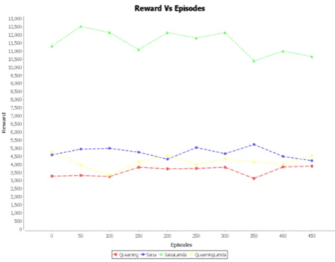
In single agent learning, the number of rewards obtained with reference to variations in episodes, discount rate, learning rate are shown in graphs. For a particular episode, Sarsa learning receives more rewards than Q-learning. An increase in the number of episodes also increases the number of rewards for both learning methods. For minimum discount rate numbers of rewards are less for both learning algorithms. For the same discount rate, numbers of rewards are more for Sarsa learning as compared to Q-learning. Single agent algorithms are implemented and results are compared. The Q function values are tabulated for obtaining some insights. Q tables show the best action (that is an optimal product) for different individual states. By knowing the Q function, the shop agent can compute best possible product for a given state that gives maximum profit to it.
Figure 1: Comparison of Rewards Vs Episodes for four algorithms Transaction
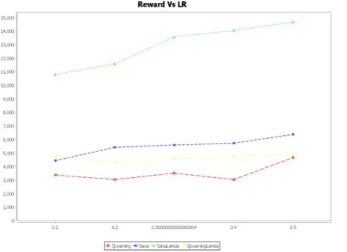
Figure 2: Comparison of Rewards Vs Discount Rate for four algorithms
Following graph shows for Single agent learning that for minimum learning rate numbers of rewards are less for both learning algorithms. For same learning rate, the numbers of
rewards are more for Sarsa learning as compared to Q-learning.
Figure 3: Comparison of Rewards Vs Discount Rate for four algorithms
In single agent learning the result analysis, is done by two different ways. Firstly, for a given month & customer age group, the product is identified. Learning shows that for a given month and an age group which products are to be selected that are best for sale. Shop agent will understand that in a month which products are to be sold to the customers having the age group. Second, it shows that in a year, the specific number of products is purchased by particular customer age group. Shop agent will understand that in a year number of products is to be sold to the customers having the
different age group. Sarsa algorithm gives better results than Q-learning and converges fast as compared to Q-learning.
CONCLUSION
Learning algorithms are best suitable for decision making. Single agent learning is the first step of development to further learning methods. It uses sequential decision making, the environment is not fully observable, less expertise with less knowledge and information. Performance is limited in the single agent system. Hence, the future work is to emphasize on the implementation of multiagent learning algorithms for the scenario to overcome the limitations in single agent learning.
REFERENCES
[1] Babak Nadjar Araabi, Sahar Mastoureshgh, and Majid Nili Ahmadabadi “A Study on Expertise of Agents and Its Effects on Cooperative Q-Learning” IEEE Transactions on Evolutionary Computation, vol:14, pp:23-57, 2010
[2] Young-Cheol Choi, Student Member, Hyo-Sung Ahn “A Survey on Multi-Agent Reinforcement Learning: Coordination Problems”, IEEE/ASME International Conference on Mechatronics and Embedded Systems and Applications, pp. 81 – 86, 2010.
[3] Zahra Abbasi, Mohammad Ali Abbasi “Reinforcement Distribution in a Team of Cooperative Q-learning Agent”, Proceedings of the 9th ACIS
International Conference on Software Engineering, Artificial Intelligence, Networking, and Parallel/Distributed Computing, IEEE Computer Society
[4] La-mei GAO, Jun ZENG, Jie WU, Min LI “Cooperative Reinforcement Learning Algorithm to Distributed Power System based on Multi-Agent” 2009 3rd International Conference on Power Electronics Systems and Applications Digital Reference: K210509035 [5] Adnan M. Al-Khatib “Cooperative Machine Learning Method” World
of Computer Science and Information Technology Journal (WCSIT) ISSN: 2221-0741 Vol.1, No.9, 380-383, 2011.
[6] Ethem Alpaydin “Introduction to Machine Learning” Second Edition, MIT Press by PHI.
[7] Tom Mitchell “Machine Learning” McGraw Hill International Edition. [8] Liviu Panait Sean Luke “Cooperative Multi-Agent Learning: The State of the Art”, published in Journal of Autonomous Agents and Multi-Agent Systems Volume 11 Issue 3, pp. 387 – 434, 05.
[9] Jun-Yuan Tao, De-Sheng Li “Cooperative Strategy Learning In Multi-Agent Environment With Continuous State Space”, IEEE International Conference on Machine Learning and Cybernetics, pp.2107 – 2111, 2006.
[10] Dr. Hamid R. Berenji David Vengerov “Learning, Cooperation, and Coordination in Multi-Agent Systems”, in Proceedings of 9th IEEE
International Conference on Fuzzy Systems, 2000.
[11] M.V. Nagendra Prasad & Victor R. Lesser “Learning Situation-Specific Coordination in Cooperative Multi-agent Systems” in Journal of Autonomous Agents and Multi-Agent Systems, Volume 2 Issue 2, pp. 173 – 207, 1999.
[12] Ronen Brafman & Moshe Tennenholtz “Learning to Coordinate Efficiently: A Model-based Approach”, in Journal of Artificial Intelligence Research, Volume 19 Issue 1, pp. 11-23, 2003.
[13] Michael Kinney & Costas Tsatsoulis “Learning Communication Strategies in Multiagent Systems”, in Journal of Applied Intelligence, Volume 9 Issue 1, pp 71-91, 1998.