Bayesian VAR Analysis in the Presence of Infrequent Shocks with Application to Analysis of Oil Price Shocks.

ABSTRACT

WENG, QIFENG. Bayesian VAR Analysis in the Presence of Infrequent Shocks with Application to Analysis of Oil Price Shocks. (Under the direction of Atsushi Inoue.)

In this paper, we propose a so-called mean-plus-noise VAR (MPNVAR) model and applied it to the macroeconomics empirical study. Along with the model, we use Bayesian approach to estimate the parameters in the model.

© Copyright 2012 by Qifeng Weng

Bayesian VAR Analysis in the Presence of Infrequent Shocks with Application to Analysis of Oil Price Shocks

by Qifeng Weng

A thesis submitted to the Graduate Faculty of North Carolina State University

in partial fulfillment of the requirements for the Degree of

Master of Science

Economics

Raleigh, North Carolina

2012

APPROVED BY:

Denis Pelletier Huixia Wang

Atsushi Inoue

DEDICATION

BIOGRAPHY

ACKNOWLEDGEMENTS

I would like to acknowledge my indebtedness to several people. First and foremost, I would like to express my gratefulness to my advisor, Dr. Atsushi Inoue. Actually, it is him who brought up this combined MPNVAR model. Without his help and guidance, this paper can not be finished. I also extend my gratitude to my advisory committee members Dr. Huixia Wang and Dr. Denis Pelletier for their insights and suggestions. I also thank all my professors in North Carolina State University.

I especially thank my grandparents Shuhua Ding and Yingjuan Shao for all what they did for me. At this time being, my grandfather Ding is struggling with his lung cancer toughly. This work is for him. I hope he will be fine soon. Then I can show it to him, making him proud of me. I love you so much, grandpa and grandma. Also I thank my parents, Liming Ding and Shijian Weng. Their support and guidance make this paper possible.

TABLE OF CONTENTS

List of Tables . . . vi

List of Figures . . . vii

Chapter 1 Introduction . . . 1

Chapter 2 Mean Plus Noise Models . . . 4

2.1 Basic Form of Mean Plus Noise Models . . . 4

2.2 Extensions of MPN Models to VAR Models . . . 5

2.3 Impulse Response Functions . . . 6

Chapter 3 Estimation Procedure. . . 7

3.1 The Likelihood Function of the Model . . . 7

3.2 Estimation ofΦ . . . 8

3.2.1 Vectorized VAR(q) model . . . 8

3.2.2 Posterior ofΦCondition on Other Parameters . . . 9

3.3 Posterior ofpCondition on Other Parameters . . . 10

3.4 Posterior ofdCondition on Other Parameters . . . 11

3.5 Posterior ofΣV Condition on Other Parameters . . . 11

3.6 Posterior ofΣ1andΣ2Condition on Other Parameters . . . 13

Chapter 4 Empirical Results . . . 14

4.1 Empirical Model and Data . . . 14

4.2 Bayesian Estimation Results for Kilian’s Trivatiate VAR Model . . . 16

4.3 Details of Parameters Estimation Procedure for MPNVAR Model . . . 17

4.4 Estimates Report . . . 18

4.5 Convergence Test Results for Mixture Model . . . 20

4.6 Monte Carlo Experiment Report . . . 21

4.7 Inference from MPNVAR model . . . 22

Chapter 5 Concluding Remarks . . . 27

LIST OF TABLES

LIST OF FIGURES

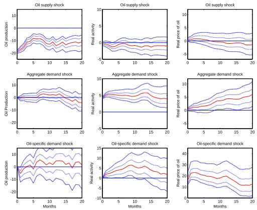
Figure 4.1 Kilian’s Trivatiate VAR Model IRF with 95% and 68% Credible Intervals (Me-dian Line in Middle) by Bayesian Estimation . . . 17 Figure 4.2 Kilian’s Historical Decomposition of Real Price of Oil Plot . . . 22 Figure 4.3 Kilian’s Historical Decomposition of Real Price of Oil Plot . . . 24 Figure 4.4 Case II: MPN Model IRF ofΣ1with 95% and 68% Credible Intervals (Median

in Middle) . . . 25 Figure 4.5 Case II: MPN Model IRF ofΣ2with 95% and 68% Credible Intervals (Median

in Middle) . . . 25 Figure 4.6 Case III: MPN Model IRF ofΣ1with 95% and 68% Credible Intervals (Median

in Middle) . . . 26 Figure 4.7 Case III: MPN Model IRF ofΣ2with 95% and 68% Credible Intervals (Median

CHAPTER

1

Introduction

forecasts than VARs estimated by the conventional approaches. Canova (1999) had specific discussions about this strength of BVAR models. Monetary policy researchers, central banker policy makers made bulk of papers going back and forth between simple univariate time series models to highly sophisticated nonlinear dynamic model for better forecast, are still in favor of Bayesian VAR.

Mean-plus-noise models have been introduced in the study of long memory and regime-switching in financial area by Chen and Tiao (1990) because of its infrequent sudden changed shocks can generate suspicious long memory behavior. This branch has been developed separately from the Bayesian VAR model. Granger and Hyung (2004) used this model to show the confusion between structural change and long memory. In an independent work, Diebold and Inoue (2000), found more general conclusions about this confusion by extending mean-plus-noise model in state space forms.

Inspired by above research and MPN model’s infrequent shock character, we see its potentials in macroeconomics filed, especially for the oil shocks study started by Kilian (2009) or other fields like monetary policy research (Uhlig, 2005). Because both oil shocks and monetary policies don’t change frequently over time. For instance, US interest rate, a benchmark of US monetary policy change, changes annually or even longer during stable economy, and quarterly or so during recession time. So monetary policy shocks occur infrequently. Major contributor to oil price changing as Kilian concluded in his paper is the precautionary demand shock. This shock presents when wars or turmoil occurs in mid-east or incident like 9/11 happens. So apparently, these shocks will not occur every day or monthly. Another feature of this infrequent shock is that once it changes, it is likely that the change will be bigger than conventional continuous disturbances and fades away in next few periods. Our MPNVAR model has the very power to handle both frequent and infrequent shocks simultaneously, which, we believe, will better describe economic phenomena like oil shocks and monetary policy. Our Monte Carlo experiment consistently verifies our belief.

The main contribution of this paper is that we proposed this new MPNVAR model and applied it to the macroeconomics empirical study. Along with the model, we use the Bayesian approach to estimate the parameters in the model. At the initial stage of this paper, we have considered the possibility to apply the MLE approach to estimate. Due to large numbers of latent variables{dt}(about 395dt’s) in our

discovered, most of parameters have conjugate distributions. Monte Carlo experiments have shown that they can be consistently estimated. Moreover, with the help of corresponding impulse response function, we show MPNVAR better explains the oil shocks.

CHAPTER

2

Mean Plus Noise Models

2.1

Basic Form of Mean Plus Noise Models

First, we introduce a multivariateMean-Plus-Noise(MPN) model, which only contains the disturbance terms. MPN model has two disturbance terms. The first one,Ut, is in a conventional form, which is

normally distributed. The second disturbance term,Vt, is also normally distributed controlled by a binary

scalar variabledt, which is from a Bernoulli distribution. It represents as below:

et n×1

= A

n×n 

 Ut

n×1

+dt 

 

Vt n1×1

0

n2×1



  



 (2.1)

where A is a (n×n) lower triangular matrix, n=n1+n2, dt is a scalar, Ut

iid

∼N(0n×1,In), Vt

iid ∼

N(0n1×1,ΣV),ΣV is a(n1×n1)diagonal matrix,dt iid

∼Bernoulli(pd).

The other way to expresset is:

et|dt

iid ∼







N(0n×1,Σ1) dt=0

N(0n×1,Σ2) dt=1

where

Σ1=AA0

Σ2=A

In1+ΣV 0n1 0n2 In2

!

A0 (2.3)

We call the first disturbance termUt asContinuous Disturbanceand the second disturbance termVt

asDiscrete Disturbance.

2.2

Extensions of MPN Models to VAR Models

Next, we extend pure MPN model to MPNVAR model by substituting conventional VAR models’ disturbance term into MPN model. We will NOT assume this process is stationary. The reason why we exclude this important assumption is that nonstationarity will not affect the following Bayesian estimation procedure, but at the same time, if included, it will bring cumbersome Bayesian estimation technique, which we try to avoid here.

We define the following system of autoregressive model whendt=1, as:

yi,t=φi,0+φi,(1)1y1,t−1+φ (1)

i,2y2,t−1+· · ·φ (1)

i,nyn,t−1 (2.4)

+φ_i,(2)₁y1,t−2+φi,(2)2y2,t−2+· · ·φ (2)

i,nyn,t−2

+· · ·+φ_i,(₁p)y1,t−p+φ( p)

i,2 y2,t−p+· · ·φ (p)

i,n yn,t−p+ui,t+dtvi,t

and whendt =0, as:

yi,t =φi,0+φ_i,(1)₁y1,t−1+φ_i,(1)₂y2,t−1+· · ·φ_i,n(1)yn,t−1 (2.5)

+φ_i,(2)₁y1,t−2+φ_i,(2)₂y2,t−2+· · ·φ_i,n(2)yn,t−2

+· · ·+φ_i,(p₁)y1,t−p+φ_i,(₂p)y2,t−p+· · ·φ_i,n(p)yn,t−p+ui,t

wherecidenotes the constant inith equation andφ

(l)

i,j denotes the coefficient of jth variable atlth time

lag in theith equation.i, j= 1,2,· · ·,nandl= 1,2,· · ·,p.

TheVAR(p)representation form of above model system is:

yt=c+Φ1yt−1+· · ·+Φpyt−p+et (2.6)

whereyt is a(n×1)vector of n observations at time t.cdenotes an(n×1)vector of constants andΦiis

a(n×n)matrix of autoregressive coefficients fori= 1,2,· · ·,p. Andet, the special disturbance term is

Further stack the equation system into aVAR(1)model, we reach:

Φ(L)Yt=c+et (2.7)

whereYt = [yp+1,yp+2,· · ·,yT]0,Φ(L)= [In, -Φ1L, -Φ2L2,· · ·, -ΦpLp], andLis the lag operator.

So far we have built the MPNVAR model. One thing we need to emphasize here is that this model can describe either stationary or nonstationary process. MPNVAR model estimation procedure by Bayesian approach will be presented in Chapter 3. Next we will show the tool that we can show MPNVAR model’s strength:Impulse Response Functions.

2.3

Impulse Response Functions

One of the major goals in this paper is to investigate whether MPNVAR model gives better interpretation of oil shocks. We are using Impulse Response Function (IRF) to measure the reaction of all variables in response to external shocks. We calculate 20 steps ahead IRF of this model. And since MPNVAR model having continuous and discrete disturbance terms, which means we’ll get two variance-covariance matrix of the error terms, we construct two separate IRF’s for each of them.

From Eq. 2.6 we first build thecompanion formof reduced-from IRF, which is:

Ψ=

"

Φ1 Φ2 · · · Φp−1 Φp

I_n·(p−1) 0n·(p−1)×n #

(2.8)

ThenJΨhJ0where row vectorJ= [In 0n×n·(p−1)], stands for thehstep ahead impulse response of

the all variables.(i,j)element of this(n×n)square sub-matrix ofΨhmeansith element ofyt in response

to the jth element ofet.

After achieving the above reduced-form IRF, we can further calculate each structural impulse response functions for this model with respect toΣ1andΣ2. Basically, according to Hamilton [9], first we get

the Cholesky decomposition ofΣ1=A−₁1A−₁1

0

andΣ2=A−₂1A−₂1

0

. Then we calculateJΨhJ0·A−₁1 and JΨhJ0·A−₂1. The two(n×n)square sub-matrix we have now are the structural impulse response function

CHAPTER

3

Estimation Procedure

3.1

The Likelihood Function of the Model

In this chapter, we implement the Bayesian method to estimate all parameters in our MPNVAR model. To use Bayesian method, the first thing we need is to get the likelihood function of the model. Since the model has similarity to the conventional VAR model, we obtain MPNVAR model likelihood function as below:

L(y|Φ,ΣV,Σ1,Σ2,d) = (2π)−3[∑ T

t=1(1−dt)]/2_| Σ1|−∑

T

t=1(1−dt)/2_exp

−1 2tr(Σ

−1

1 (M1·et)

0_·

(M1·et))

× (2π)−3[∑ T

t=1dt]/2_|Σ

2|−∑

T

t=1dt/2_exp

−1 2tr(Σ

−1

2 (M2·et)0·(M2·et))

× (1−p)∑Tt=1(1−dt)_×p∑Tt=1dt _(3.1)

whereet=Φ(L)Yt−c;M2=diag({dt}),the diagonal elements ofM2are from{dt}, others are 0’s;M1=

Or same likelihood in another expression:

L(y|Φ,ΣV,Σ1,Σ2,d) = (2π)−3[∑ T

t=1(1−dt)]/2_| Σ1|−∑

T

t=1(1−dt)/2_{exp −}1

2

T

∑

t=1

[(1−dt)e0tΣ

−1 1 et]

!

× (2π)−3[∑ T t=1dt]/2_|

Σ2|−∑

T

t=1dt/2_{exp −}1

2

T

∑

t=1

[dtet0Σ

−1 2 et]

!

× (1−p)∑Tt=1(1−dt)_×p∑Tt=1dt _(3.2)

whereet =Yt−Φ(L)Yt−1,Σ1andΣ2are defined in Eq. 2.3.

The reason why we give out two forms of likelihood function is that these two forms of likelihood function will be required during the derivation of different parameters’ posterior distribution.

With the likelihood function of this model, we can implement Bayesian method to estimate each parameter sequentially in this model. we estimate the parameters in the following order: slope coefficients matrixΦ(L)orΦ, probability parameterpin the Bernoulli distribution, latent variable{dt}, variance

matrixΣV in discrete disturbance terms andΣ1.Σ2is determined byΣV andΣ1. This will not lose the

generality since later we use the Gibbs Sampler method to simulate these estimates iteratively.

3.2

Estimation of

Φ

We impose the prior of Φ which is multivariate normally distributed (Φ0 ∼N(µΦ,ΣΦ)), where ΣΦ

is considered as given. Since the likelihood function is similar to multivariate normal likelihood, the posterior ofΦlikely have a conjugate distribution. The proof is showed in below.

First, we clean up the likelihood function, only keeping the terms havingΦ, which would be:

exp

−1 2tr(Σ

−1_(M

1·et)0·(M1·et))

·exp

−1 2tr(Σ

−1

2 (M2·et)0·(M2·et))

For the convenience of deriving the posterior ofΦ, mainly for dealing with the Kronecker operator,

we first need to vectorize the whole equation system and use the technique below.

3.2.1 Vectorized VAR(q) model

In previous section we have built our VAR(1) model as:

Yt =Φ(L)Yt−1+et et= 





ut∼N(0,Σ1) dt=0

vt∼N(0,Σ2) dt=1

Since later we need to use vectorized VAR(1) model to achieve the posterior ofΦ, referring to Canova’s

notes (2010) [2], we let y=vec(Yt), X = [yt−1,· · ·,yt−p],Φ=vec(Φ(L)) ande=vec(et). Then the

vectorized VAR(1) model would be:

y= (I3⊗X)Φ+e e∼N(0,Σ1⊗M1+Σ2⊗M2) (3.4)

wherey,eare (n·T×1) vectors,I3is the identify matrix, andΦis a(n·(n·p+1)×1)vector.

M1=IT−diag({dt})andM2=diag({dt})

Then the likelihood function would be:

L(y|Φ,Σ1,Σ2,d) =

1

(2π0.5·nT)|Σ1⊗M1+Σ2⊗M2|

−0.5 _(3.5)

×exp{−0.5(y−(I3⊗X)Φ)0(Σ−₁1⊗M1+Σ−₂1⊗M2)(y−(I3⊗X)Φ)}

where:d={d₁,d2,· · ·,dT}

Now we can make some manipulations of the likelihood function focusing on terms havingΦ:

(y−(I3⊗X)Φ)0(Σ−₁1⊗M1+Σ−₂1⊗M2)(y−(I3⊗X)Φ)

=(Σ−₁0.5⊗M1+Σ₂−0.5⊗M2)·(y−(I3⊗X)Φ)0·(Σ−₁0.5⊗M1+Σ₂−0.5⊗M2)·(y−(I3⊗X)Φ)

=(∆y−ΞΦ)0(∆y−ΞΦ)

where ∆= (Σ−₁0.5⊗M1+Σ−20.5⊗M2) Ξ= (Σ1−0.5⊗M1+Σ2−0.5⊗M2)(I3⊗X)

Also (∆y−ΞΦ) =∆y−ΞΦˆ +Ξ(Φˆ −Φ)

where Φˆ = ((Σ−₁1⊗M1+Σ−21⊗M2)⊗X0X)−1((Σ−11⊗M1+Σ−21⊗M2)⊗X)y

3.2.2 Posterior ofΦCondition on Other Parameters

In this paper we are going to use f0(·)to denote the prior pdf and f1(·)as the posterior pdf. Now we can

explicitly write out the prior ofΦ0∼N(Φ¯,ΣΦ),which is:

f0(Φ)∝|ΣΦ|

−0.5_exp[−0.5(

Φ−Φ¯)0Σ−_Φ1(Φ−Φ¯)]

=|ΣΦ|

−0.5_exp[−0.5(

Then the posterior ofΦwould be proportional to the product of likelihood and prior:

f1(Φ|y;Θ)∝g(Φ)L(y|Φ;Θ)

∝exp[−0.5(Σ−_Φ0.5(Φ−Φ¯))0Σ_Φ−0.5(Φ−Φ¯)]×exp(∆y−ΞΦ)0(∆y−ΞΦ)

=exp{−0.5[(Φ−Φ∗)0Z0Z(Φ−Φ∗) + (z−ZΦ∗)0(z−ZΦ∗)]} (3.7)

where:

z= [Σ−_Φ0.5·Φ0 ∆y]0 (3.8)

Z= [Σ−_Φ0.5 Ξ]0 (3.9)

Φ∗= (Z0Z)−1(Z0z) (3.10)

where ∆= (Σ−₁0.5⊗M1+Σ−20.5⊗M2), Ξ= (Σ1−0.5⊗M1+Σ2−0.5⊗M2)(I3⊗X)

SinceΣ1,Σ2andΣΦare fixed, the second term above is a constant and

f1(Φ|y)∝exp[−0.5(Φ−Φ∗)0Z0Z(Φ−Φ∗)]

∝exp[−0.5(Φ−Φ∗)0(Σ∗_Φ)−1(Φ−Φ∗)] (3.11)

So Posterior ofΦis:

Φ1∼N(Φ∗,Σ∗_Φ)

Φ∗= (Z0Z)−1(Z0z) Σ∗_Φ= (Z0Z)−1 (3.12)

3.3

Posterior of

p

Condition on Other Parameters

To estimate parameter p, we impose prior distribution of parameter pas beta distribution. So the pdf of Beta distribution is as below:

f₀(p) = Γ(α+β)

Γ(α)Γ(β)p

α−1_(1−p)β−1 _(3.13)

Use the same way as we did in last section, we get the posterior of f₁(p|Φ,Σ1,Σ2,d)is proportional

to the product of likelihood and its prior:

f1(p|Φ,d,ΣV,Σ1,Σ2)∝pα−1+∑

T

Obviously, the posterior ofpis still conventional Beta distribution.

p₁∼Beta(α+ T

∑

t=1

dt,β+ T

∑

t=1

(1−dt)) (3.15)

3.4

Posterior of

d

Condition on Other Parameters

d denotes as{dt;t=1,2,· · ·,T}. Unlike we did before, sincedare latent variables in this model, we

need to reorganize the model likelihood function (Eq. 3.2) only keep the terms havingd. Then we have the posterior ofdis:

f₁(d|Φ,p,ΣV,Σ1,Σ2)∝[A(1−p)]T−∑

T

t=1dt·_[B(p)]∑Tt=1dt _(3.16)

where

A= (2π)−3/2[∑ T

t=1(1−dt)]_|

Σ|−1/2∑ T

t=1(1−dt)_{exp −}1

2

T

∑

t=1

[(1−dt)e0tΣ

−1_e

t] !

B= (2π)−3/2[∑ T t=1dt]|_Σ

2|−1/2∑

T

t=1dt_exp −1 2

T

∑

t=1

[dtet0Σ−21et] !

(3.17)

Or:

f1(d|Φ,p,ΣV,Σ1,Σ2)∝







2π−

3 2 · |_Σ2|−

1 2·p

·exp −1₂·e_t0Σ−₂1et

ifdt =1

2π−

3 2 · |_Σ|−

1

2 ·(1−p)

·exp −1 2·e

0

tΣ−1et

ifdt =0

(3.18)

Where:et =Yt−Φ(L)Yt−1. Obviously, the posterior ofdis still conventional Bernoulli distribution by

normalizing above posterior pdf function.

3.5

Posterior of

Σ

Condition on Other Parameters

To estimateΣV, we first need to filter the likelihood function to keep those terms havingΣV. Although we

ofΣ2in Eq. 3.2 and substitute it with the form ofΣV in Eq. 2.3:

g(y|Φ,ΣV,Σ1,Σ2,d)

=

A In1+σV 0n1 0n2 In2

! A0

−∑Tt=1dt/2

exp



−

1 2tr(A

0−1 In1+σV 0n1 0n2 In2

!−1

A−1(M2·et)0·(M2·et))   =

In1+σV 0n1 0n2 In2

!

−∑Tt=1dt/2

exp



−

1 2tr(A

0−1 In1+σV 0n1 0n2 In2

!−1

A−1(M2·et)0(M2·et)) 

 (3.19)

Then we impose a Inv-Wishart prior toΣV to draw its posterior. Following is the general pdf form of

Wishart and inv-Wishart distribution for the use of drawing posterior ofΣV. Assume the prior distribution

of parameterΣ−1follows Wishart distribution f(Λ;n,Σ). Its pdf is as below:

f(Λ;n,Σ) = |Λ|

(n−d−1)/2_{exp(−(1/2)tr(}

ΛΣ−1))

2dn/2_πd(d−1)/4_|Σ|n/2_∏d

i=1Γ((n+1−i)/2)

(3.20)

whereΛ=∑Na=1(Xa−X¯)(Xa−X)¯ 0 is a scale matrix in the pdf,d is the dimension ofΣ,Xa

iid

∼N(µ,Σ)

|Λ|=det(Λ),|Σ|=det(Σ)and f(Λ;n,Σ) =0 unlesswis symmetric and positive definite

SubstituteΣ_V−1into Eq. 3.20, we have Σ−_V1∼Wishart(n,Λ−1), which is equivalent toΣV ∼Inv− Wishart. Its pdf is:

f₀(Σ_V−1;n,Λ−1) = |ΣV|

−(n−d−1)/2_{exp(−(1/2)tr(}

Σ_V−1Λ))

2dn/2_πd(d−1)/4_|Λ|−n/2

∏di=1Γ((n+1−i)/2)

(3.21)

where|ΣV|=det(ΣV),dis the dimension ofΣ,|Λ|=det(Λ),n=∑tT=1dt and f(ΣV−1,n,Λ−1) =0 unless Σ_V−1is symmetric and positive definite.

The Posterior of f1(ΣV|Φ,p,d,Σ1,Σ2)is proportional to the product of likelihood and its prior:

f1(ΣV|Φ,p,d,Σ1,Σ2)∝|ΣV|−(∑

T

t=1dt−3−1)/2_{exp(−(1/2)tr(Σ}−1 V Λ))

×

In1+ΣV 0n1 0n2 In2

!

−∑Tt=1dt/2

exp



−

1 2tr(A

0−1 In1+ΣV 0n1 0n2 In2

!−1

A−1(M2·et)0(M2·et)) 

 (3.22)

whereΛ=tr((A−1M2·et)(A−1M2·et)0+I3)whereΣ1=AA0.

3.6

Posterior of

Σ

and

Σ

Condition on Other Parameters

Because of the relationship betweenΣ1andΣ2, once we estimatedΣ1,Σ2is also estimated. So to keep

the proof as simple as possible, we only write out the posterior distribution ofΣ1. Use the same pdf of

Wishart distribution expressed above (Eq. 3.21). The Posterior of f₁(Σ1|Φ,p,d)is proportional to the

product of likelihood and its prior:

f₁(Σ1|Φ,p,d,ΣV)∝|Σ1|−(n0−3−1)/2exp

−1 2tr(Σ

−1 1 Λ0)

×

|Σ1|−∑

T

t=1(1−dt)/2_exp −1 2

T

∑

t=1

[(1−dt)et0Σ−11et] !

×

|Σ2|−∑

T

t=1dt/2_exp −1 2

T

∑

t=1

[dte0tΣ−21et] !

(3.23)

whereet=Yt−Φ(L)Yt−1,n0=∑Tt=1(1−dt),Λ0=ete0t/(n0−np−1). KeepingΣ2is becauseΣ2relates

toΣ1.

CHAPTER

4

Empirical Results

4.1

Empirical Model and Data

This paper is building on the work of Kilian (2009) [10]. We use processed data set from Kilian’s paper and the same structural VAR(24) model to reach our results to compare it with Kilian’s. To compare our Bayesian estimation results of MPNVAR model with his, we make a change in Kilian’s estimation process that is instead of implementing bootstrap as Kilian did in his paper, we use Bayesian method to estimate his conventional VAR(24) model. This change allows us to compare two different results on the same paper.

We inherit Kilian’s structural VAR(24) regression model with replaced new disturbance terms (MPN) to obtain our empirical MPNVAR model as (Eq. 4.1). This structural model is a little different from the reduced form VAR(p) model as we described in the last chapter for the structural coefficient matrixA0.

After some manipulation, it is easy to convert the structural model to reduced form model. Then we can follow the estimation procedure we developed previously to make inference of this model. In this particular case, the model system contains 3 variables. They are thepercent change in global crude oil productiondenoted as∆prodt, the loggedindex of real economic activitycalculated by Kilian denoted as

reat and the logged and deflatedreal oil price r pot. The VAR model extends top=24 time lags. The

to each of the shock factor independently. Hence the empirical MPNVAR models are:

Case I: A0yt =c+

24

∑

j=1

Ajyt−j+Ut+ 

 

dtvt1

0 0





 (4.1)

Case II: A₀yt =c+

24

∑

j=1

Ajyt−j+Ut+ 

 

0 dtvt2

0





 (4.2)

Case III: A₀yt =c+

24

∑

j=1

Ajyt−j+Ut+ 

 

0 0 dtvt3





 (4.3)

whereUt

iid

∼N(03×1,I3),vti

iid

∼N(0,σ_vi2),dt

iid

∼Bernoulli(pd).

Ut denotes the vector of serially and mutually uncorrelatedcontinuous structural innovationsand

vt’s denotes the corresponding discrete shocks in each independent model, i.e.vt1denotesdiscrete oil

supply shock,vt3denotesdiscrete aggregate demand shockandvt3denotesdiscrete oil specific-demand

shock. They are all indexed by a binary variabledt which indicates if an infrequent event triggers

discrete oil shocks. Like what Kilian did in his paper, we postulate thatA−₀1 has a recursive structure such that the reduced form errorset can be decomposed according toet=A−₀1Ut+dtA−₀1Vt by labeling

A−₀1=A=



 

a₁₁ 0 0 a21 a22 0

a31 a32 a33





. So we have:

Case I:

et≡ 

 

e∆prodt t

ereat_t er pot

t   =   

a11 0 0

a21 a22 0

a31 a32 a33

        

utcons oil supply shock

u_tcons aggregate demand shock ucons oil speci f ict −demand shock



 +dt



 

vt1

0 0       (4.4)

whereΣ1=A−₀1A−₀1

0

,Σ2=A−₀1



 

1+σv2 0 0

0 1 0

0 0 1

  A −1 0 0 . Case II:

et≡ 

 

e∆prodt t

ereat t

er pot t   =   

a11 0 0

a21 a22 0

a₃₁ a₃₂ a₃₃

        

utcons oil supply shock

utcons aggregate demand shock

ucons oil speci f ic_t −demand shock



 +dt



 

0 vt2

whereΣ1=A−₀1A−₀1

0

,Σ2=A−₀1



 

1 0 0

0 1+σv2 0

0 0 1

  A −1 0 0 . Case III:

et≡ 

 

e∆prodt t

ereat_t etr pot

  =   

a₁₁ 0 0 a21 a22 0

a31 a32 a33

        

u_tcons oil supply shock u_tcons aggregate demand shock ucons oil speci f ict −demand shock



 +dt



 

0 0 vt3

      (4.6)

whereΣ1=A−01A

−1 0

0

,Σ2=A−01



 

1 0 0

0 1 0

0 0 1+σv2   A −1 0 0 .

By multiplyingA−₀1 on both sides of the structural VAR(24) models, we can achieve the reduced form VAR(24) models to implement the estimation method we developed in the previous chapter:

yt=c+

24

∑

j=1

Φjyt−j+eti i=1,2,3 (4.7)

where Φj =A−₀1Aj,t=1,2,· · ·,395 and this reduced form model (Eq. 4.7) is the same as Eq. 2.6.

The corresponding parameters in Eq. 2.7 are: n=3, p=24,T =419−p=395, theΦj is a(3×3)

matrix,yt is a(3×1)matrix andetihereby is a(3×1)matrix. Now we finally build our reduced form

MPNVAR(24) model.

4.2

Bayesian Estimation Results for Kilian’s Trivatiate VAR Model

0 5 10 15 20 -20

-10 0 10

Oil supply shock

Oil production

0 5 10 15 20 -5

0 5 10

Oil supply shock

Real activity

0 5 10 15 20 -5

0 5 10

Oil supply shock

Real price of oil

0 5 10 15 20 -20

-10 0 10

Aggregate demand shock

Oil Production

0 5 10 15 20 -5

0 5 10

Aggregate demand shock

Real activity

0 5 10 15 20 -5

0 5 10

Aggregate demand shock

Real price of oil

0 5 10 15 20 -20

-10 0 10

Oil-specific demand shock

Oil production

Months

0 5 10 15 20 -5

0 5 10

Oil-specific demand shock

Real activity

Months

0 5 10 15 20 -5

0 5 10

Oil-specific demand shock

Real price of oil

Months

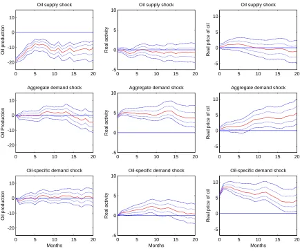
Figure 4.1: Kilian’s Trivatiate VAR Model IRF with 95% and 68% Credible Intervals (Median Line in Middle) by Bayesian Estimation

4.3

Details of Parameters Estimation Procedure for MPNVAR Model

After this preparation, we move forward to estimate our innovative MPNVAR model. All three cases are estimated in the same way. We follow the procedure in chapter 3. Here we give out all details about setups, priors we use, etc.

Before the MCMC step, we setup all initial parameters value by their corresponding OLS estimated values. For theΦprior, we useΦOLS as its mean, and build a(219×1)variance matrix with random

numbers in uniform distribution from 1 to 10 automatically generated by MATLAB built-in function. With the prior we can easily generate random values fromΦ’s posterior distributionN(Φ∗,Σ∗_Φ), then

p’s posterior distribution is straightforward. We simply use MATLAB built-in Beta function to generate random variables by settingα =6 andβ =8. We tried many other value, this combination

makes convergence speed faster than smaller values and seems more reasonable than bigger values. And these initial values setting also helps avoiding getting extremeσvvalue.

With updated information ofΦ, new residuals andp, we generatedseries one by one from a binomial

function in MATLAB using normalized parameter. By saying normalizing, we calculate corresponding values ofAandBin Eq. 3.17, and then set fractionB/(A+B)as the probability parameter in binomial distribution.

Forσvwe use Metropolis-Hastings algorithm to draw random variables from the messy posterior pdf.

One thing needs to be mentioned is that since this particular model has 24 lags and 395 time periods, they cause over-float issues in MATLAB when we calculate some powers in the expression. So we first take the log to avoid over-float issue, then take the exp at the accept-reject step in Metropolis-Hastings. And the jumping distribution we choose here is simply uniform distribution.

Last parameters we estimate areΣ1andΣ2. We use pretty much the same approach as we did in the

σvstep for their similarity except for the choice of jumping distributions we use. During the exploration

of the jumping distribution, we find that the biggest contributor to the log(·)value of the posterior is from

the −(n0−3−1)

2 log(det(Σ1))term, which is 1000 times larger than the log value of the rest terms. So to

eliminate this effect we impose jumping the distribution’s pdf to be:

Jt(θ∗|θ(t−1))

Jt(θ(t−1)|θ∗)

=exp(det(Σ

(t−1) 1 ))

n0−np−1 exp(det(Σ∗₁))n0−np−1

whereΣ∗₁denotes the candidate ofΣ1andΣ(

t−1)

1 denotes the most recent acceptedΣ1draw.

Along with each iteration of parameter estimation, we record the structural impulse response functions of the model with continuously updated parameters we simulated before.

4.4

Estimates Report

Table 4.1 shows the estimates after 25,000 draws (first 10% draws discarded) from the Gibbs Sampler method for each case. Note that since the slope coefficient matrixΦcontains 219 elements, giving out all estimates of them is not helpful. The estimate we show below is a(3×3)matrix averaged over all time lags. Its expression is:

ˆ¯

Φ= 1

24

24

∑

j=1

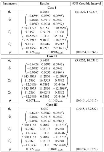
Table 4.1: MPNVAR Model Estimates (Posterior Mean)

Parameters Results 95% Credible Interval

Case I

ˆ

σv 8.2567 (4.0229, 17.7276)

ˆ¯

Φ





−0.6594 0.0292 0.0695 −0.0484 0.9719 0.0749 −0.0360 0.0031 0.9857

  ˆ Σ1  

353.1727 5.3157 −10.5550 5.3157 17.9109 1.0338 −10.5550 1.0338 35.1841

  ˆ Σ2  

715.3917 9.1030 −18.8757 9.1030 18.0416 0.9212 −18.8757 0.9212 223.8713





ˆ

p 0.0699mean 0.0506mode (0.0254, 0.1366)

Case II

ˆ

σv 5.9403 (3.7262, 10.5315)

ˆ¯

Φ





−0.6929 0.0282 0.0743 −0.0487 0.9718 0.0742 −0.0367 0.0032 0.9864

  ˆ Σ1  

345.5075 11.2860 −12.5989 11.2860 16.5503 0.5892 −12.5989 0.5892 37.4496

  ˆ Σ2  

345.5075 11.2860 −12.5989 11.2860 80.6248 0.5892 −12.5989 0.5892 37.4496





ˆ

p 0.1071mean 0.1013mode (0.0401, 0.1915)

Case III

ˆ

σv 8.042 (3.945, 18.2527)

ˆ¯

Φ





−0.6929 0.0282 0.0743 −0.0487 0.9718 0.0742 −0.0367 0.0032 0.9864

  ˆ Σ1  

360.1163 5.7069 −11.3732 5.7069 17.8107 0.9248 −11.3732 1.0332 34.8246

  ˆ Σ2  

360.1163 5.7069 −11.3732 5.7069 17.8107 0.9248 −11.3732 1.0332 266.4268





ˆ

4.5

Convergence Test Results for Mixture Model

After achieving tens of thousands of draws to estimate the parameters in this model, we need to make sure all estimates have come to convergence when we stop the simulation procedure. Since we iteratively get the draws by implementing Gibbs Sampler method, these draws can be considered as time series data. To assess whether or not these estimates have converged to the desired posterior distribution in a certain finite sample, we use theconvergence diagnosis (CD) testdeveloped by Geweke (1992) [7]. Following is Geweke’s CD test algorithm. We haveθ1denotes the first subsample, which having totalT1draws andθ2

from the second subsample which havingT2draws. From Geweke’s paper,T1is the first 10% ofMdraws.

Mhere is draws after discarding first 10% burn-in period of the original data draws.T2is the bottom 50%

ofMdraws. Geweke found that ifT₁/MandT₂/Mare fixed, and(T1+T2)/M<1, then asM→∞then:

¯

θ1−θ¯2

p

Avar(θ¯1)/T1+Avar(θ¯2)/T2

⇒N(0,1) (4.8)

whereAvar(θ¯1)andAvar(θ¯2)are the long-run asymptotic variance ofθ1andθ2. And their estimates are

defined as below:







ˆ

Avar(θ¯1) =Γˆ (1) 0 +2∑

K1

j=1(1−

j K1+1)

ˆ

Γ(1)_j

ˆ

Avar(θ¯2) =Γˆ(2)₀ +2∑Kj=12 (1−

j K2+1)

ˆ

Γ(2)_j

(4.9)

In the Eq. 4.9, ˆΓ(_ji)denotes the consistent estimate for thejth sample auto-covariance matrix in theith

subsample set.(1−_Kj

i+1)is calledBartlett Kernel. and theKiis theBandwidthfor the CD test. Literature

shows that the CD statistics are sensitive to the choice of both Bartlett Kernel and Bandwidth. And the choice of Bandwidth is the key for the test. In this thesis we use the method of choosing bandwidth has been brought by Newey and West (1994) [14]. There are also other methods available to choose the bandwidth. Here is how we apply Newey and West’s automatic bandwidth selection method:

ˆ

Γ(_ji)= (1/T(i))

T_(i)

∑

t=j+1

(θt(i)−θ¯( i)₎₍

θ_t(₋i)_j−θ¯(i))

n= [4(T(i)/100)2/9]

ˆ sa=2

n

∑

j=1

jΓˆ(_ji) sˆb=Γ

(i) 0 +2

n

∑

j=1

ˆ

Γ(_ji)

ˆ

γ=1.1447({sˆa/sˆb}2)1/3

K₍i)= [γˆ·T 1/3

(i) ] (4.10)

We have theH0hypothesis: parameter simulated by Gibbs Sampler method are converged in certain

finite samples. And we calculate the convergence test statistic forθ by:

CD(θ) =

¯

θ1−θ¯2

p

Avar(θ¯1)/T1+Avar(θ¯2)/T2

(4.11)

If |CD(θ)| is greater than 1.96, we reject theH0hypothesis with Type I errorα=5%. If not then we fail

to reject theH0hypothesis with Type I errorα=5%.

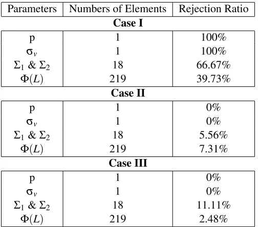
With above test method, we ran the convergence test for each of the parameters in our MPN model with significant level 5% (22,500 draws left after burn-in period). Table 4.2 shows the results:

Table 4.2: Convergence Test Results

Parameters Numbers of Elements Rejection Ratio

Case I

p 1 100%

σv 1 100%

Σ1&Σ2 18 66.67%

Φ(L) 219 39.73%

Case II

p 1 0%

σv 1 0%

Σ1&Σ2 18 5.56%

Φ(L) 219 7.31%

Case III

p 1 0%

σv 1 0%

Σ1&Σ2 18 11.11%

Φ(L) 219 2.48%

Since HAC test will over-reject more than 5% and there are only small amount of elements in the first two parameters, our test result meets our expectation quite well. So we can say our estimates have converged after 25,000 replications of MCMC method.

4.6

Monte Carlo Experiment Report

estimates of simulated data. Compare them with results showed in section 4.4 to see if they are reasonably close. The Monte Carlo experiment results (Table 4.3) reasonably indicate that the estimation procedure is plausible:

4.7

Inference from MPNVAR model

From the estimation results, case I is not reasonable. First reason is that, the supply disturbance is quite stable according to the historic data. The estimation results are more frequent than expected. The other reason why we drop it is that the estimates never converge in our convergence test. Case II and Case III’s results meet our initial anticipation. We make inference from Case II and Case III only.

For Case II: After achieving consistently estimated parameters, we analyze them in this section.

We found that ˆpmean=0.1071 and ˆpmode=0.1013. This means, by monthly frequency data, discrete

oil specific shocks occasionally occur every 9.3 month (by mean). And the other important parameter isσv=5.9. 5.9 means the discrete disturbance is about 6 times larger than the continuous shocks. As

you can see in Figure 4.2 (oil specific-demand shocks plot), if we count peaks beyond +0.29 and -0.29

1975 1980 1985 1990 1995 2000 2005

-0.5 0 0.5

Aggregate Oil Shock

Figure 4.2: Kilian’s Historical Decomposition of Real Price of Oil Plot

bound as the discrete disturbance, we get 40 peaks, which is about every 10.2 month one big shock. This approximately matches our 9.3 month frequency in mode sense. +0.29 and -0.29 bound is calculated from±((+1−(−1))/7) =±0.29.

We use Σ1 andΣ2 to build corresponding impulse response function for each case. Figure 4.4 is

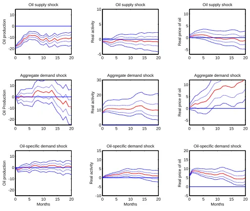
the IRF plot of continuous disturbance terms in our Mean plus Noise model by ignoring the discrete error term over all time period, i.e. same disturbance in Kilian’s model and Figure 4.5 is the IRF plot of discrete disturbance terms over all time period, i.e. at each time period, the oil shocks having both frequent and infrequent shock factors.

Table 4.3: Monte Carlo Experiment Estimates (Posterior Mean)

Parameters Estimated Results 95% Credible Interval

Case I

d

(σv)MC 4.3045 (2.3346, 6.3487)

d

(Φ)MC





−1.4361 −0.0587 0.1006 0.2341 0.9930 0.0299 −0.1505 −0.0079 0.9895





d

(Σ1)MC 



337.3448 24.2653 −15.5950 24.2653 24.2759 −3.4370 −15.5950 −3.4370 48.5735





d

(Σ2)MC





145.69 104.2 −68.0 104.2 30.3 −7.3 −68.0 −7.3 51.7





ˆ

p 0.0618mean 0.0506mode (0.0224, 0.1145)

Case II

d

(σv)MC 8.4251 (4.6504, 14.6052)

d

(Φ)MC





−1.2300 −0.0020 −0.1515 0.0391 0.9204 0.0430 −0.0858 −0.0016 0.9863





d

(Σ1)MC 



389.1351 16.8761 −33.0577 16.8761 20.6361 8.0430 −33.0577 8.0430 50.1577





d

(Σ2)MC 



389.1351 16.8761 −33.0577 16.8761 191.6584 8.0430 −33.0577 8.0430 50.1577





ˆ

p 0.0608mean 0.0481mode (0.0294, 0.1049)

Case III

d

(σv)MC 6.265 (3.157, 10.650)

d

(Φ)MC





−1.2035 0.0450 −0.0476 −0.1826 0.9586 0.0777 −0.0342 0.0093 0.9767





d

(Σ1)MC 



357.7975 27.2786 −10.8794 27.2786 23.7256 −2.1590 −10.8794 −2.1590 37.8577





d

(Σ2)MC 



357.7975 27.2786 −10.8794 27.2786 23.7256 −2.1590 −10.8794 −2.1590 209.2842





ˆ

that plot is also consistent as our assumption that discrete innovation is only on oil specific-demand shocks. Because only bottom 3 subplots have dramatic difference from the original model’s IRF. The band width is about 4 times lager thanΣ1’s, noticing that we change the y-axis scale in theΣ2’s IRF plot.

However, the shocks forecast behaviors are very similar in these two IRF plots. Each of them has the correspondingly same curve.

For Case III: After achieving consistently estimated parameters, we analyze them in this section.

We found that ˆp_mean=0.066 and ˆp_mode=0.048. This means, by monthly frequency data, discrete oil specific shocks occasionally occur every 1.7 years (by mode). And the other important parameter is

σv=8.0. 8.0 means the discrete disturbance is about 8 times larger than the continuous shocks. As

you can see in Figure 4.3 (oil specific-demand shocks plot), if we count peaks beyond +0.11 and -0.11

1975 1980 1985 1990 1995 2000 2005 -1

-0.5 0 0.5 1

Oil Supply Shock

1975 1980 1985 1990 1995 2000 2005 -1

-0.5 0 0.5 1

Aggregate Demand Shock

1975 1980 1985 1990 1995 2000 2005 -1

-0.5 0 0.5 1

Oil-Specific Demand Shock

Figure 4.3: Kilian’s Historical Decomposition of Real Price of Oil Plot

bound as the discrete disturbance, we get 21 peaks, which is about every 1.6 year one big shock. This approximately matches our 1.7 year frequency in mode sense. +0.11 and -0.11 bound is calculated from ±((+1−(−1))/9) =±0.11.

We use Σ1 andΣ2 to build corresponding impulse response function for each case. Figure 4.6 is

the IRF plot of continuous disturbance terms in our Mean plus Noise model by ignoring the discrete error term over all time period, i.e. same disturbance in Kilian’s model and Figure 4.7 is the IRF plot of discrete disturbance terms over all time period, i.e. at each time period, the oil shocks having both frequent and infrequent shock factors.

Σ1’s IRF is basically the same thing as Bayesian results of Kilian’s original model. And no wonder

that plot is also consistent as our assumption that discrete innovation is only on oil specific-demand shocks. Because only bottom 3 subplots have dramatic difference from the original model’s IRF. The band width is about 4 times lager thanΣ1’s, noticing that we change the y-axis scale in theΣ2’s IRF plot.

0 5 10 15 20 -20

-10 0 10

Oil supply shock

Oil production

0 5 10 15 20 -5

0 5

10 Oil supply shock

Real activity

0 5 10 15 20 -5

0 5 10

Oil supply shock

Real price of oil

0 5 10 15 20 -20

-10 0 10

Aggregate demand shock

Oil Production

0 5 10 15 20 -5

0 5 10

Aggregate demand shock

Real activity

0 5 10 15 20 -5

0 5 10

Aggregate demand shock

Real price of oil

0 5 10 15 20 -20

-10 0 10

Oil-specific demand shock

Oil production

Months

0 5 10 15 20 -5

0 5

10 Oil-specific demand shock

Real activity

Months

0 5 10 15 20 -5

0 5 10

Oil-specific demand shock

Real price of oil

Months

Figure 4.4: Case II: MPN Model IRF ofΣ1with 95% and 68% Credible Intervals (Median in Middle)

0 5 10 15 20 -20

-10 0 10

Oil supply shock

Oil production

0 5 10 15 20 -5

0 5 10

Oil supply shock

Real activity

0 5 10 15 20 -5

0 5 10

Oil supply shock

Real price of oil

0 5 10 15 20 -20

-10 0 10

Aggregate demand shock

Oil Production

0 5 10 15 20 0

10 20

30 Aggregate demand shock

Real activity

0 5 10 15 20 -5

0 5 10

Aggregate demand shock

Real price of oil

0 5 10 15 20 -20

-10 0 10

Oil-specific demand shock

Oil production

Months

0 5 10 15 20 -10 -5 0 5 10 15

Oil-specific demand shock

Real activity

Months

0 5 10 15 20 -5 0 5 10 15 20

Oil-specific demand shock

Real price of oil

Months

0 5 10 15 20 -20

-10 0 10

Oil supply shock

Oil production

0 5 10 15 20 -5

0 5 10

Oil supply shock

Real activity

0 5 10 15 20 -5

0 5 10

Oil supply shock

Real price of oil

0 5 10 15 20 -20

-10 0 10

Aggregate demand shock

Oil Production

0 5 10 15 20 -5

0 5

10 Aggregate demand shock

Real activity

0 5 10 15 20 -5

0 5 10

Aggregate demand shock

Real price of oil

0 5 10 15 20 -20

-10 0 10

Oil-specific demand shock

Oil production

Months

0 5 10 15 20 -5

0 5 10

Oil-specific demand shock

Real activity

Months

0 5 10 15 20 -5

0 5 10

Oil-specific demand shock

Real price of oil

Months

Figure 4.6: Case III: MPN Model IRF ofΣ1with 95% and 68% Credible Intervals (Median in Middle)

0 5 10 15 20 -20

-10 0 10

Oil supply shock

Oil production

0 5 10 15 20 -5

0 5

10 Oil supply shock

Real activity

0 5 10 15 20 -5

0 5 10

Oil supply shock

Real price of oil

0 5 10 15 20 -20

-10 0 10

Aggregate demand shock

Oil Production

0 5 10 15 20 -5

0 5 10

Aggregate demand shock

Real activity

0 5 10 15 20 -5

0 5 10

Aggregate demand shock

Real price of oil

0 5 10 15 20 -20

-10 0 10

Oil-specific demand shock

Oil production

Months

0 5 10 15 20 -10

-5 0 5 10

15 Oil-specific demand shock

Real activity

Months

0 5 10 15 20 0

10 20 30 40

Oil-specific demand shock

Real price of oil

Months

CHAPTER

5

Concluding Remarks

We propose MPNVAR model in structura and reduced VAR forms and apply them to the study of oil shocks. We find that oil specific-demand shock is the biggest contributor to the oil price fluctuation, it roughly occurs every 1.7 years. And the magnitude of this discrete shock is about 8 times of conventional continuous shock. This conclusion matches the historical data in Kilian (2009).

REFERENCES

[1] Fabio Canova. Vector Autoregressive Models: Specification, Estimation, Inference and Forecasting, volume Volume 1:, page 482. Wiley-Blackwell, 1999.

[2] Fabio Canova. Bayesian var models. Unpublished Note, 2010.

[3] Chung Chen and George C. Tiao. Random level-shift time series models, arima approximations, and level-shift detection. Journal of Business & Economic Statistics, 8(1):pp. 83–97, 1990.

[4] Siddhartha Chib and Edward Greenberg. Hierarchical analysis of sur models with extensions to correlated serial errors and time-varying parameter models. Journal of Econometrics, 68(2):339 – 360, 1995.

[5] Francis X. Diebold and Atsushi Inoue. Long memory and regime switching. Journal of Economet-rics, 105(1):131 – 159, 2001.

[6] Alan E. Gelfand, Susan E. Hills, Amy Racine-Poon, and Adrian F. M. Smith. Illustration of bayesian inference in normal data models using gibbs sampling. Journal of the American Statistical Association, 85(412):pp. 972–985, 1990.

[7] John Geweke. Evaluating the accuracy of sampling-based approaches to the calculation of posterior moments. Technical report, 1991.

[8] Clive W.J. Granger and Namwon Hyung. Occasional structural breaks and long memory with an application to the sp 500 absolute stock returns. Journal of Empirical Finance, 11(3):399 – 421, 2004.

[9] James D. Hamilton. Time Series Analysis. Princeton University Press, 1994.

[10] Lutz Kilian. Not all oil price shocks are alike: Disentangling demand and supply shocks in the crude oil market. American Economic Review, 99(3):1053–69, 2009.

[11] Robert Litterman. Forecasting with bayesian vector autoregressions – five years of experience: Robert b. litterman, journal of business and economic statistics 4 (1986) 25-38. International Journal of Forecasting, 2(4):497–498, 1986.

[12] Robert B. Litterman. Techniques of forecasting using vector autoregressions. Technical report, 1980.

[13] Nicholas Metropolis, Arianna W. Rosenbluth, Marshall N. Rosenbluth, Augusta H. Teller, and Edward Teller. Equation of state calculations by fast computing machines. The Journal of Chemical Physics, 21(6):1087–1092, 1953.

[14] Whitney K Newey and Kenneth D West. Automatic lag selection in covariance matrix estimation. Review of Economic Studies, 61(4):631–53, October 1994.

[16] Christopher A. Sims. Money, income, and causality. The American Economic Review, 62(4):pp. 540–552, 1972.

[17] Christopher A. Sims. Macroeconomics and reality. Econometrica, 48(1):pp. 1–48, 1980.

[18] Christopher A. Sims and Tao Zha. Were there regime switches in u.s. monetary policy? The American Economic Review, 96(1):pp. 54–81, 2006.

[19] Harald Uhlig. Bayesian vector autoregressions with stochastic volatility. Econometrica, 65(1):pp. 59–73, 1997.