Volume 2011, Article ID 121787,11pages doi:10.1155/2011/121787
Research Article
Multistrategy Self-Organizing Map Learning for
Classification Problems
S. Hasan and S. M. Shamsuddin
Soft Computing Research Group, Faculty of Computer Science and Information System, Universiti Teknologi Malaysia, Skudai, 81300 Johor, Malaysia
Correspondence should be addressed to S. M. Shamsuddin,[email protected]
Received 12 January 2011; Revised 21 April 2011; Accepted 23 June 2011
Academic Editor: Francois Benoit Vialatte
Copyright © 2011 S. Hasan and S. M. Shamsuddin. This is an open access article distributed under the Creative Commons Attribution License, which permits unrestricted use, distribution, and reproduction in any medium, provided the original work is properly cited.
Multistrategy Learning of Self-Organizing Map (SOM) and Particle Swarm Optimization (PSO) is commonly implemented in clustering domain due to its capabilities in handling complex data characteristics. However, some of these multistrategy learning architectures have weaknesses such as slow convergence time always being trapped in the local minima. This paper proposes multistrategy learning of SOM lattice structure with Particle Swarm Optimisation which is called ESOMPSO for solving various classification problems. The enhancement of SOM lattice structure is implemented by introducing a new hexagon formulation for better mapping quality in data classification and labeling. The weights of the enhanced SOM are optimised using PSO to obtain better output quality. The proposed method has been tested on various standard datasets with substantial comparisons with existing SOM network and various distance measurement. The results show that our proposed method yields a promising result with better average accuracy and quantisation errors compared to the other methods as well as convincing significant test.
1. Introduction
In classification process; normally, large classes of objects are separated into smaller classes. This approach can be very complicated due to the challenge in identifying the criteria especially for procedures involving complex data structures. In this scenario; practically, the Machine Learning (ML) techniques will be used and introduced by many researchers as alternative solutions to solve the above problems. Among the ML methods and tools, Artificial Neural Network (ANN), Fuzzy Set, Genetic Algorithm (GA), Swarm Intelli-gence (SI), and rough set are commonly used by researchers. However, the most popular ML method widely used by the practitioners is ANN [1]. Various applications of ANN which have been implemented in many practical problems such as meteorological forecasting, image processing, and agriculture are discussed in [2–4]. In ANN model, simple neurons are connected together to form series of connected network. While a neural network does not have to be adapt-ive, its advantages arise with proper algorithms to update the weights of the connections to produce a desired output.
ANN and evolutionary computation methodologies have each been proven effective in solving certain classes of prob-lems. For example, neural networks are very efficient at map-ping input to output vectors and evolutionary algorithms are very useful at optimization. ANN weaknesses could be solved either by enhancing the structures of ANN itself or by hybridizing it with evolutionary optimisation [5,6]. Evolu-tionary computation is based on population of optimisation techniques such as evolutionary Algorithm (EA) and Swarm Intelligence (SI). One of the techniques used in EA is Genetic Algorithm (GA), inspired by biological evolution such as inheritance, mutation, selection, and crossover. On the other hand, SI methods such as Particle Swarm Optimisation (PSO) and Ant Colony Optimisation (ACO) are motivated by flock of birds, swarm of bees, ant colony, and school of fish.
technique called PSO which requires little computational costs. The authors argued that PSO could train Feedforward Neural Network (FNN) with a performance similar to the backpropagation (BP) method, for the XOR and Iris bench-marks. Since then, several researchers have adopted PSO for FNN learning. However, most of the studies focus on the hybridisation of PSO and FNN. Few studies have been conducted on the hybridisation of PSO with Self-Organizing Map (SOM) to solve complex problems.
Early studies have shown that the multistrategy learning of PSO-SOM approach was first introduced by Shi and Eberhart [8] with modified particle swarm optimizer. Subse-quently, Xiao et al. [9,10] used hybrid SOM-PSO approach to produce better clustering of gene datasets. The authors used SOM learning and PSO to optimise the weights of SOM. However, the merit for combination of SOM-PSO without conscience factor was poor than SOM alone. This is because this factor is valuable as a competitive learning technique, but it reduces the number of epochs necessary to produce a ro-bust solution. In 2006, O’neill and Brabazon [11] adopted PSO as unsupervised SOM algorithm. The authors suggested using different distance metric in calculating the distance be-tween input vectors and each member of the swarm to pro-duce competitive result for data classification. However, in this study, types of SOM lattice structure were not con-sidered.
Moreover, Chandramouli [12] used SOM and PSO for image classifier, and the author stated that SOM was domi-nant in image classification problems. However, the problem emerged in generating image classes which provided concise visualisation of the image dataset. Therefore, the author used dual layer of SOM structure and PSO to optimise the weights of SOM neurons. In addition, Forkan and Shamsuddin [13] introduced a new method for surface reconstruction based on hybridization of SOM and PSO. The authors used grow-ing grid structure in the Kohonen network to learn the sam-ple data through mapping grid and PSO to probe the opti-mum fitting points on the surface. In this study, the proposed Kohonen network was a 3D rectangular map and being en-hanced using growing grid method. However, this study did not focus on the lattice structure of the Kohonennetwork.
Sharma and Omlin [14] utilized a U-matrix of SOM to determine cluster boundaries using PSO algorithm. The au-thors compared the results with other clustering techniques such as k-means and hierarchical clustering. However, this study did not focus on the structure of SOM architecture. Recently, ¨Ozc¸ift et al. [15] proposed PSO in the optimisation of SOM algorithm to reduce the training time without loss of quality in clustering. The author stated that the size of lattice is related to the clustering quality of SOM. This optimisation technique has successfully reduced the numbers of nodes that finds the best-matching unit (BMU) for a particular input. Having a larger grid size in SOM will invite higher training time. Furthermore, the larger the lattice size, the more nodes should be considered for BMU calculation, thus causes higher operating cost for the algorithm.
Since 1993, Extension of SOM network topologies such as self-organization network has been implemented in many applications. Fritzke [16] introduced Growing Cell
Struc-tures (GCS) for unsupervised learning in data visualisation, vector quantization and clustering, while supervised GCS is suitable for data classification with Radial Basis Function (RBF). In 1995, Fritzke extended the growing neural gas to dynamic SOM known as Growing SOM (GSOM). Hsu et al. [17] stated that GSOM can provide balance performance in topology preservation, data visualization, and computational speed. Consequently, Chan et al. [18] used GSOM to improve binning process and later Forkan and Shamsuddin [13] for intelligent surface reconstruction.
Hybridization of SOM and evolutionary method was proposed by Cr´eput et al. [19] to address the vehicle routing problem with time windows. In this study, the experimental result shows that the proposed method improves SOM-based neural network application. In addition, Khu et al. [20] implemented the combination of multiobjective GA and SOM to incorporate multiple observations for distributed hydrologic model calibration. SOM clustering has reduced the number of objective functions while multiobjective GA was implemented to give better solution in optimization problems. Furthermore, Eisuke [21] investigated GA per-formance by combining GA with SOM to improve search performance by real-coded GA (RCGA). The result shows that SOM-GA gives better solution in computation times rather than RCGA.
The quality of the Kohonen map is determined by its lat-tice structure. This is because the weights for each neuron in the neighborhood will be updated by these lattice structures. There are many types of SOM lattice structures: circle lattice structure, rectangular, hexagonal, spherical (Figure 1), and torus (Figure 2). Many studies have been done on comparing the lattice structure of SOM, for instance, between traditional SOM and Spherical [22,23].
Spherical and Torus SOM representing the plane lattice give a better view of the input data as well as provide closer links to edge nodes. They make the 2D visualisation of multi-variate data possible using SOM’s code vectors as data source [24]. Spherical and Torus SOM structures focus on topolog-ical grid mapping structures rather than improvement on lattice structure. This is due to the border effect issues that were highlighted in previous studies by Ritter [25] Marzouki and Yamakawa [26]. Furthermore, the usefulness of the Spherical SOM for clustering and visualization is discussed in [27,28].
According to Middleton et al. [29], hexagonal lattice structure is effective for image processing since the structure can uniform the image pixel. Park et al. [30] has used the hexagonal lattice to provide better visualization. Hexagonal lattice was preferred because it does not favor horizontal or vertical directions [31]. The number of nodes was deter-mined as 5×number of samples [32]. Basically, the two largest eigenvalues of the training data were calculated, and the ratio between the side lengths of the map grid was set to the ratio between the two maximum eigenvalues. The actual side lengths were set so that the product was close to the determined number of map units.
Figure 1: Spherical SOM [24].
approach with cluster and Principal Component Analysis (PCA) for large environmental dataset. The results obtained allowed detecting natural clusters of monitoring locations with similar water quality type and identifying important discriminant variables responsible for the clustering. SOM clustering allows simultaneous observation of both spatial and temporal changes in water quality.
Wu and Takatsuka [34] used fast spherical SOM for ge-odesic data structure. The proposed method was used to remove border effect in SOM, but the limitation was slower in computation times. Furthermore, Kihato et al. [24] imple-mented spherical and torus SOM for analysis, visualization, and prediction of the syndrome trends. The proposed meth-od has been implemented by physicians to monitor patients’ current health trends and status.
Due to limitations of the previous studies focusing on the improvement of SOM lattice structure, this study enhanced SOM lattice structure with improved hexagonal lattice area. In SOM competitive learning process, wider lattice are need-ed for searching the winning nodes as well as for weights ad-justment. This allows SOM to get a good set of weights for improving the quality of data classification and labeling. Par-ticle Swarm Optimisation (PSO) is developed to optimize SOMs’ training weights accordingly. The hybridisation of SOM-PSO architecture, so-called Enhanced SOM with Par-ticle Swarm Optimisation (ESOMPSO) is proposed with im-provement on the lattice structure for better classification. The performance of the proposed ESOMPSO is validated based on the classification accuracy and quantization errors (QE). The error deviations between the proposed methods are computed to further illustrate the efficiency of these ap-proaches accordingly.
2. The Proposed Method
In this study, we proposed multistrategy learning with the Enhancement of SOM with PSO (ESOMPSO) and improved formulation of hexagonal lattice structure. Unlike conven-tional hexagonal lattice (as given in (1)), a neighbourhood of the proposed formulation is given with the influence of
N(j,t) instead of the neighbourhood width,N(j). SinceD(t) is a threshold value, it will decrease gradually as training
Figure 2: Torus SOM. http://altnett.ning.com/profiles/blogs/the-sphere.
progresses. For this neighbourhood function, the distance is determined by considering the distance of each dimension. The dimension with the maximum value is chosen as distance node from BMU,d(j).N(j) corresponds to a hex-agonal lattice aroundnwin having neighbourhood width as below:
R=6×1
2×r×
(r2)−
1 4r2
, (1)
whereRis the standard hexagonal lattice and
Nj,t=
⎧ ⎨ ⎩
1,dj≤D(t)
0,dj> D(t). (2)
The weights of all neurons within this hexagon are up-dated withN(j)=1, while the others remaining unchanged. As the training progresses, this neighborhood gets smaller, resulting in the neurons that are very close to the winner and will get updated accordingly. The training stops when there is no more neuron in the neighborhood. Usually, the neighborhood function,N(j,t), is chosen as an L-dimen-sional Gaussian function as given below:
Nj,t=exp−d
j2
2σ(t)2 . (3)
The proposed SOM algorithm for the above process is shown below.
For each input vectorV, do the following.
(a) Initialisation—set initial synaptic weights to small random values, say in a interval [0, 1], and assign a small positive value to the learning rate parameter. (b) Competition—for each output node j, calculate
the value D(V −Wj) of the scoring function. For
instance, Euclidean distance measurement is denoted as
DV−Wj
=
i=n
i=0
Vi−Wi j
2
radius = n, bmu (x, y), right border x = bmu x; left border x = bmu x; right border y = bmu y + 2∗n; left border y = bmu y−2∗n; Up right border x = bmu x−n; Up right border y = bmu y + n; Bottom right border x = bmu x + n; Bottom right border y = bmu y + n; Up left border x = bmu x – n; Up left border y = bmu y−n; Bottom left border x = bmu x + n; Bottom left border y = bmu y−n;
Algorithm 1: Algorithm for improved hexagonal lattice area.
for the Manhattan distance, the equation is given as
DV−Wj
=
i=n
i=0
Vi−Wi j
, (4b)
for the Chebyshev distance, the equation is given as
DV−Wj
=max
i
Vi−Wi j. (4c)
Find the winning nodeJthat minimizesD(V−Wj)
overall output nodes.
(c) Cooperation—identify all output nodes jwithin the neighborhood ofJdefined by the neighborhood size
R. For these nodes, do the following for all input records. Reduce the radius with exponential decay function:
σ(t)=σ0exp
−1
λ
, t=1, 2, 3,. . ., (5)
where σ0 is the initial radius, λ is the maximum iteration,tis the current iteration; and formulation of improved hexagonal lattice is given as
Rnew=(2r+ 1)2+ 2r2, (6)
where Rnew is the enhanced/improved hexagonal lattice,ris the neighborhood radius.
(d) Adaptation—adjust the weights:
W(t+ 1)=W(t) +Θ(t)L(t)(V(t)−W(t)), (7)
whereLis the learning rate,Θis the influence a node’s distance from the BMU,
L(t)=L0exp
−t
λ
, t=1, 2, 3,. . ., (8)
whereL0is the initial learning rate,
Θ(t)=exp
− dist 2
2σ2(t)
, t=1, 2, 3. . ., (9)
and dist is the distance of a node from BMU,σis the width of neighborhood.
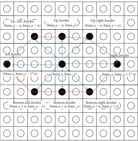
Up left border
(bmux−n, bmuy−n)
Up right border
(bmux−n, bmuy+n)
Bottom left border
(bmux+n, bmuy−n) (bmuBottom right borderx+n, bmuy+n)
right border left border
Up border
(bmux−n, bmuy)
Bottom border
(bmux+n, bmu y)
(bmux, bmu y) (bmux, bmuy+ 2∗n)
(bmux, bmuy−2∗n)
Figure 3: The proposed lattice structure for enhanced SOM
(ESOM).
(e) Iteration—adjust the learning rate and neighbor-hood size, as needed until no changes occur in the feature map. Repeat step (ii) and stop when the ter-mination criteria are met. The improved hexago-nal lattice area consists of six important points: right border (x,y), left border (x,y), up right bor-der (x,y), up left border (x,y), bottom right border (x,y), bottom left border (x,y) (see Algorithm1).
Figure 3illustrates the formulation of improved
hex-agonal lattice area. Detail explanation of the proposed method is discussed in next paragraph.
Shi in 1995 [35]. PSO is a global optimisation, population-based evolutionary algorithm for dealing with problems in which the best solution can be presented as a point or surface in ann-dimensional space. Hypothesis are plotted
in this space and seeded with an initial velocity, as well as a communication between the particles. In this study, the hybridisation approach of ESOMPSO is based on the Koho-nen structure to improve the quality of data classification and labeling. An improved hexagonal lattice area is introduced for SOM learning enhancement; and PSO is integrated into this proposed SOM to evolve the weights for the learning prior to the weights adjustments. This is because PSO can find the best reduced search space for a particular input and support the algorithm to take more nodes into consideration while determining search space and not to be trapped by the same node continuously [15]. The algorithm for integrating ESOMPSO is shown below. At this stage, the enhanced SOM will be implemented for the classification purpose to obtain the weights and later will be optimised using PSO.
(1) The rectangular topology and hexagonal lattice struc-ture of the SOM is initialized with feastruc-ture vectorsmi,
wherei=1, 2,. . .,Krandomly, whereKis the length of the feature vector.
(2) Input feature vectorxis presented to the network and the winner nodeJ, that is closest to the input pattern,
xis chosen using the equation:
J=argiminx−mj
. (10)
(3) Initialise the population array of particle representing random solutions forddimensional problem space. (4) For each particle, the distance function is evaluated,
Di j= k
l=1
xi j−xjl. (11)
(5) The personal best pbest is updated by the following condition:
iffpbesti
>currenti
, then pbesti=currenti. (12)
(6) The global best gbest is updated with the following condition:
iffgbestd
=f(currentd)
, thengbestd=currentd.
(13)
(7) Update the velocityVidusing
Vid=WxVid+C1
Gbest,d−Xid
+C2Pbest,i−Xid
, (14) whereC1 > 0 andC2 > 0 constants are called the
cognitive and social parameters, and W > 0 is a constant called the inertia parameter.
(8) Update the positionXidusing
Xid=Xid+Vid, (15)
whereXid is the new positionXandVid is the new
velocityV.
(9) Repeat steps 2 to 9 until all input patterns are ex-hausted in the training.
3. Experimental Setup
To investigate the effectiveness of PSO in evolving the weights from SOM, the proposed method has been performed in the testing and validation process. In the testing phase, data is presented to the network with target nodes for each input sets. The reference attributes or classifier computed during training process is used to classify input data set. The algorithm identifies the winning node that will be used for determining the output of the network. Then, the output of the network is compared to the expected result to decide the ability of the network for classification phase. This classification stage will classify test data into correct predefined classes obtained during training process. A num-ber of data is presented to the network, and the percentage of correct classified data is calculated. The percentage of the correctness is measured to obtain the accuracy and the learning ability of the network. The result is validated and compared using several performance measurements: quantisation error (QE) and classification accuracy. Later, the error differences between the proposed methods are computed for further validations.
The performance measurement of the proposed methods is based on quantisation error (QE) and classification accura-cy (CA). QE is measured after SOM’s training, and CA is the analysis for testing. The efficiency of the proposed methods is validated accordingly; if QE values are smaller and the classification accuracy is higher, then the results are prom-ising. QE is used for measuring the quality of SOM map. QE of an input vector is defined by the difference between the input vector and the closest codebook vectors. QE describes how accurately the neurons respond to the given dataset. For example, if the reference vector of the BMU calculated for a given testing vectorxi is exactly similar asxi, the error in
precision is 0.0. The equation is given as follows Quantization Error:
Eq=
1
N
N
k−1
xk(t)−wmk(t), (16)
wherewmkis the best unit of weight on timest.
While the classification accuracy indicates how well the classes are separated on the map, the classification accuracy of new samples measures the networks generalisation for better quality of SOM’s mapping.
Classification accuracy,
P(%)= n
N×100, (17)
wheren is the number of classified pattern, N is the total number of testing data.
Table 1: Data information.
Data type Iris XOR Cancer Glass Pendigits
Input node 4 4 30 10 16
Output ode 1 1 1 1 1
Data size 150 8 569 214 10992
Training size 120 6 379 149 494
Testing size 30 2 190 65 498
give better accuracy despites higher convergence time. As PSO and improved lattice structure are being implemented, the convergence time is increasing. This scenario is due to the PSO process in searching for thegbest of BMU as well as wider coverage for updating nodes with the improved lattice structure.
Self-Organizing Maps (SOM) has two layers: input and output layers. The basic SOM architecture consists of a lattice that acts as an output layer with its input nodes fully connected. In this study, the network architecture is designed based on the selected real world classification problems.
Table 1provides the specification for each dataset.
The input layer is comprised of input pattern with dif-ferent nodes that is randomly chosen from training data set. Input patterns are presented to all output nodes (neurons) in the network simultaneously. The number of input node determines the number of data required to be fed into the network, while the numbers of nodes in the Kohonen layer represent the maximum number of possible classes.
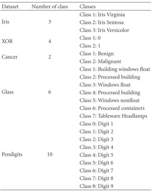
Table 2shows the class information for Iris, XOR, Glass, and
Pendigits training datasets.
The training starts once the dataset has been initialised and input patterns have been selected. The learning phase of the SOM algorithm repeatedly presents numerous patterns to the network. The learning rule of the classifier allows these training cases to organize in a two-dimensional feature map. Patterns which resemble each other are mapped onto a specific cluster. During the training phase, the class for randomly selected input node is determined. This is done by labeling the output node that is more similar (best-matching unit) to the input node compared to other nodes in the Kohonen mapping structure. The outputs from the training are the resulting map that contains the winning neurons and its associated weight vectors. Subsequently, these weight vectors are optimised by PSO. The quality of the classification accuracy is calculated to investigate the behavior of the network in the training data.
In the testing phase, for any input patterns, if themth neuron is the winner, it belongs to themth clusters. In this case, we were able to test the capacity of the network to correctly classify new independent test set to a reasonable class. An independent test set is a set similar to the input set but not part of the training set. The testing set can be seen as a representative of the general case. There is no weight updating in the recalling phase. A series of datasets obtained that was not used in learning phases, but was previously interpreted, was presented to the network. For each case, the response of the network (the label of the associated neuron) was compared to the expected result, and the percentage
Table 2: Class information.
Dataset Number of class Classes
Iris 3
Class 1: Iris Virginia Class 2: Iris Sentosa Class 3: Iris Versicolor
XOR 4 Class 1: 0
Class 2: 1
Cancer 2 Class 1: Benign
Class 2: Malignant
Glass 6
Class 1: Building windows float Class 2: Processed building Class 3: Windows float Class 4: Processed building Class 5: Windows nonfloat Class 6: Processed containers Class 7: Tableware Headlamps
Pendigits 10
Class 0: Digit 1 Class 1: Digit 2 Class 2: Digit 3 Class 3: Digit 4 Class 4: Digit 5 Class 5: Digit 6 Class 6: Digit 7 Class 7: Digit 8 Class 8: Digit 9
of correct responses was computed. This simulation results obtained from standard SOM and Enhanced SOM classifiers were used for further analysis.
It is often reported in the literature that the success of the Self-Organizing Maps (SOM) formation is critically dependent on the initial weights and the selection of main parameters of the algorithm, namely, the learning rate pa-rameter and the neighborhood set [36,37]. They usually have to be counteracted by trial and error method, hence time consuming to retrain the procedures. Due to the time con-straints, all the parameter values were fixed and constantly used throughout all the experiments. According to [38], the number of map units is usually in the range of 100 to 600. Deboeck and Kohonen [39] recommend using ten times the dimension of the input patterns as the number of neurons, and this was adopted in these experiments.
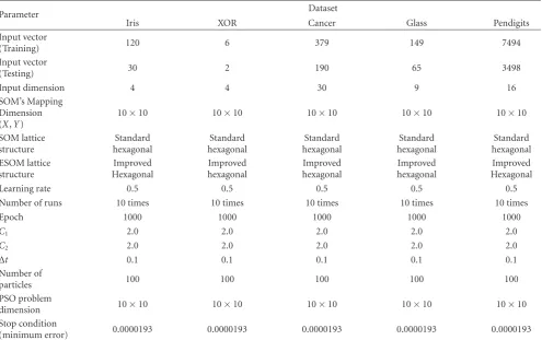
Table 3: Parameter settings for ESOMPSO.
Parameter Dataset
Iris XOR Cancer Glass Pendigits
Input vector
(Training) 120 6 379 149 7494
Input vector
(Testing) 30 2 190 65 3498
Input dimension 4 4 30 9 16
SOM’s Mapping Dimension (X,Y)
10×10 10×10 10×10 10×10 10×10
SOM lattice structure
Standard hexagonal
Standard hexagonal
Standard hexagonal
Standard hexagonal
Standard hexagonal ESOM lattice
structure
Improved Hexagonal
Improved hexagonal
Improved hexagonal
Improved hexagonal
Improved Hexagonal
Learning rate 0.5 0.5 0.5 0.5 0.5
Number of runs 10 times 10 times 10 times 10 times 10 times
Epoch 1000 1000 1000 1000 1000
C1 2.0 2.0 2.0 2.0 2.0
C2 2.0 2.0 2.0 2.0 2.0
Δt 0.1 0.1 0.1 0.1 0.1
Number of
particles 100 100 100 100 100
PSO problem
dimension 10×10 10×10 10×10 10×10 10×10
Stop condition
(minimum error) 0.0000193 0.0000193 0.0000193 0.0000193 0.0000193
a more natural mapping so as to help the algorithm converge in a more stable manner.
The accuracy of the map also depends on the number of iterations of the SOM algorithm. A rule of thumb states, for good statistical accuracy, number of iterations should be at least 500 times the number of neurons. According to [36], the total learning time is always 100 to 10000. If the time taken is longer, the clustering result becomes inaccurate. A more serious problem is that the topology preserving mapping is not guaranteed even if a huge number of iterations were used. Here, the SOM classifiers were evaluated by measur-ing the performance of clustermeasur-ing result based on the clas-sification accuracy and the computation time [41]. To meet the requirement of SOM’s quality measurement, the quanti-sation error was calculated, which is defined as the average distance between every input vector and its BMU. The ex-periments on ESOMPSO were carried out for each selected dataset (Table 3).
4. Experimental Results and Analysis
The experiments were conducted with various datasets and distance measurements: Euclidean, Manhattan, and Cheby-shev distance. The comparisons were conducted between standard SOM and standard SOM with improved hexagonal structure, so-called ESOM. Standard SOM was trained using standard hexagonal lattice, while ESOM with improved
hexagonal lattice. The choice of distance measure influen-ces the accuracy, efficiency, and generalisation ability of the results. From Table 4, ESOM with Euclidean distance gives promising accuracy of 86.9876%, followed by the Chebyshev distance 84.2561% and the Manhattan distance 80.4462%. The least quantisation error is 0.0108 for Glass dataset. It shows that the improved lattice structure of ESOM yields significant impact on the accuracy of the classifica-tions.
Table 4: Summarization of SOM and ESOM results.
SOM ESOM
EUC MAN CHEBY EUC MAN CHEBY
IRIS Quantization error 0.0348 0.0358 0.0419 0.0171 0.0244 0.0275
Classification (%) 74.3333 60.0000 70.0000 76.6667 73.3333 74.333
XOR Quantization error 0.2009 0.2060 0.2159 0.1941 0.2458 0.2077
Classification (%) 75.3436 68.4525 72.5632 86.9876 80.4462 84.2561
CANCER Quantization error 0.4541 0.4913 0.5037 0.4397 0.4771 0.4781
Classification (%) 37.8947 43.1579 74.2105 77.8947 34.7368 71.5789
GLASS Quantization error 0.0337 0.0307 0.0350 0.0108 0.0122 0.0117
Classification (%) 50.9231 13.8462 36.9231 55.3846 50.7692 44.6154
PENDIGITS Quantization error 0.1986 0.2006 0.2103 0.1897 0.1957 1.2008
Classification (%) 74.6427 44.5969 72.6415 76.3579 52.9445 69.1252
EUC: Euclidean distance, MAN: Manhattan distance, CHEBY: Chebyshev distance.
Table 5: Summarisation of SOMPSO and ESOMPSO results.
SOMPSO ESOMPSO
EUC MAN CHEBY EUC MAN CHEBY
Iris
Epoch 1000 1000 1000 1000 1000 1000
Quantisation error 4.0799 4.0979 4.0875 1.8884 2.0125 2.0565
Convergence error 0.0318 0.0358 0.0322 0.0243 0.0587 0.0347
Convergence time 22 sec 22 sec 22 sec 240 sec 240 sec 240 sec
Classification (%) 92.00 89.24 90.45 92.72 90.11 90.75
XOR
Epoch 1000 1000 1000 1000 1000 1000
Quantisation error 0.5011 0.6455 0.5866 0.0048 0.0250 0.0145
Convergence error 0.2500 0.3204 0.3050 0.1916 0.2591 0.2641
Convergence time 10 sec 10 sec 10 sec 17 sec 17 sec 17 sec
Classification (%) 94.11 85.25 88.47 95.22 86.14 90.24
Cancer
Epoch 1000 1000 1000 1000 1000 1000
Quantisation error 0.0094 0.0145 0.0102 0.0050 0.0125 0.0078
Convergence error 0.5951 0.6523 0.6424 0.4422 0.5371 0.4823
Convergence time 80 sec 80 sec 80 sec 110 sec 110 sec 110 sec
Classification (%) 90.69 75.23 78.89 91.77 77.35 82.05
Glass
Epoch 1000 1000 1000 1000 1000 1000
Quantisation error 0.0046 0.0087 0.0052 0.0038 0.0060 0.0048
Convergence error 0.0435 0.0541 0.1242 0.0157 0.0324 0.0224
Convergence time 40 sec 40 sec 40 sec 60 sec 60 sec 60 sec
Classification (%) 87.88 80.98 84.66 89.45 82.45 84.87
Pendigits
Epoch 1000 1000 1000 1000 1000 1000
Quantization error 0.0458 0.4752 0.4777 0.0587 0.5143 0.4221
Convergence error 0.2060 0.2365 0.2241 0.1405 0.1569 0.1478
Convergence time 110 sec 110 sec 110 sec 205 sec 205 sec 205 sec
Classification (%) 75.44 70.25 72.48 85.62 70.85 72.89
EUC: Euclidean distance, MAN: Manhattan distance, CHEBY: Chebyshev distance.
Figures4and5depict the effectiveness of the ESOMPSO with better average accuracy and quantisation errors com-pared to the others. Regardless the types of distance meas-urements, the results of the proposed method are significant. This is due to the improved lattice structure and PSO in optimising the weights. As discussed before, the improved formulation of the hexagonal lattice structure gives more coverage on neighbourhood updating procedure. Hence, the probability for searching the salient nodes as winner
nodes is higher, and this is presented in terms of accuracy and quantisation. However, the convergence time is slower for the proposed method due to the natural behaviour of the particles in searching for gbest globally and locally. ESOMPSO with Euclidean distance gives the highest classi-fication accuracy of 95.22% and the least quantisation error of 0.0038, accordingly.
Table 6: Kruskal-Willis ranks for the proposed methods.
Methods Number of datasets Mean rank based on accuracy (Euclidean distance)
Mean rank based on accuracy (the Manhattan distance)
Mean rank based on accuracy (the Chebyshev distance)
SOM 5 3.60 4.60 6.00
ESOM 5 8.40 7.60 7.00
SOMPSO 5 14.20 14.40 13.80
ESOMPSO 5 15.80 15.40 15.20
Total 20
P-value 0.004 0.008 0.025
0 20 40 60 80 100
SOM ESOM SOMPSO ESOMPSO
A
ve
ra
ge
ac
cur
acy
(%)
Model
Euclidean Manhattan Chebyshev 75.34
86.99 94.11 95.22
68.45
80.45 89.24 90.11
74.21
84.26 90.45 91.75
10 30 50 70 90
Figure 4: Accuracy SOM, ESOM, SOMPSO, and ESOMPSO.
SOM ESOM SOMPSO ESOMPSO
Model
Euclidean Manhattan Chebyshev 0
0.005 0.01 0.015 0.02 0.025 0.03 0.035 0.04
Av
er
ag
e
o
f
er
ro
r
0.0337
0.0108
0.0046 0.0038 0.0307
0.0122
0.0087
0.006 0.035
0.0117
0.0052 0.0048
Figure 5: Quantization errors of SOM, ESOM, SOMPSO, and
ESOMPSO.
the success of the proposed methods due to the concept of
No Free Lunch Theorem [42]. It means that general-purpose universal algorithm is impossible; an algorithm may be good at one class of problems, but its performance will suffer in the other problems. For detail explanation, higher accuracy is depending not only on types of datasets but also on the purpose of implementing the problems’ undertaking.
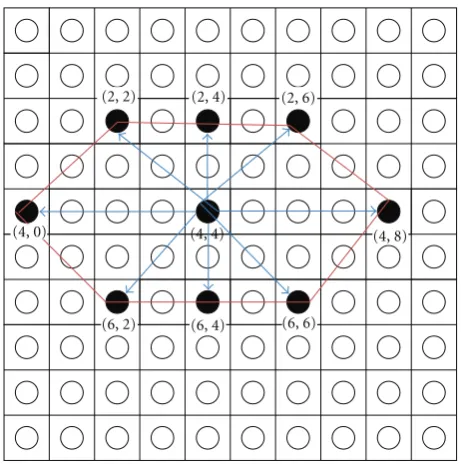
From the findings, it seems that the selection of SOM’s lattice structure for better learning is crucial in updating the neighbourhood structures for network learning. The stand-ard formulation for basic and improved hexagonal lattice structure is illustrated inFigure 6. However, after training, the number of nodes to be updated was 10.39. Using the
(4, 4) (4, 8)
(4, 0)
(2, 2) (2, 4) (2, 6)
(6, 2) (6, 4) (6, 6)
Figure 6: Improved hexagonal lattice structure.
basic hexagonal formula, the wide area was not covered and caused insufficient neighborhood updating. The potential node might not be counted during the updating process. Now, we illustrate the scenario of the improved hexagonal lattice structure for wider and better coverage (Figure 6). Let say the BMU coordinate is (4, 4) with current radius,r =2. The radius will decrease with exponential decay function. The improved neighborhood hexagonal lattice area is defined as (2).
The generatedPvalue is 0.004 which is less than the level of significant value ofα=0.05. Hence, the proposed methods have shown their dissimilarity among each other.
5. Conclusion
This paper presents multistrategy learning by proposing Enhanced Self-Organizing Map with Particle Swarm Opti-mization (ESOMPSO) for classification problems. The pro-posed method was successfully implemented on machine learning datasets: XOR, Cancer, Glass, Pendigits, and Iris. The analysis was done by comparing the results for each dataset produced by Self-Organising Map (SOM), Enhanced Self-Organising Map (ESOM), Self-Organizing Map with Particle Swarm Optimization (SOMPSO) and ESOMPSO with different distance measurements. The analysis reveals that ESOMPSO with Euclidean distance generate promising results based on the highest accuracy and the least quan-tization errors (referring to Figures 5 and6) compared to SOM, ESOM, and SOMPSO for classification problems. This major impact of the proposed method is due to the improved formulation of the hexagonal lattice structure which gives more distributions and wider exploration and exploitation of the particle swarm optimization (PSO) particles to search for a bettergbest.
Acknowledgments
Authors would like to thank the Research Management Centre (RMC), Universiti Teknologi Malaysia, and the Soft
Computing Research Group (SCRG) for the support in
making this studies a success.
References
[1] M. Negnevitsky, Artificial Intelligence: A Guide to Intelligent
Systems, Addison Wesley, Harlow, England, 2nd edition, 2005.
[2] S. Chattopadhyay, D. Jhajharia, and G. Chattopadhyay, “Uni-variate modelling of monthly maximum temperature time series over northeast India: neural network versus Yule-Walker equation based approach,” Meteorological Applications, vol. 18, no. 1, pp. 70–82, 2011.
[3] Y. L. Wong and S. M. Shamsuddin, “Writer identification for Chinese handwriting,” International Journal of Advances in Soft
Computing and Its Applications (IJASCA), vol. 2, no. 2, 2010.
[4] S. Hasan and M. N. M. Sap, “Pest clustering with self organ-izing map for rice productivity,” International Journal of
Ad-vances in Soft Computing and Its Applications (IJASCA), vol. 2,
no. 2, 2010.
[5] S. M. Shamsuddin, M. N. Sulaiman, and M. Darus, “An improved error signal for the backpropagation model for clas-sification problems,” International Journal of Computer
Math-ematics, vol. 76, no. 3, pp. 297–305, 2001.
[6] C. Surajit and B. Goutami, “Artificial neural network with backpropagation learning to predict mean monthly total ozone in Arosa, Switzerland,” International Journal of Remote
Sensing, vol. 28, no. 20, pp. 4471–4482, 2007.
[7] J. Kennedy and R. C. Eberhart, “Particle swarm optimization,” in Proceedings of the International Conference on Neural
Net-works, vol. 4, pp. 1942–1948, IEEE service center, Piscataway,
NJ, USA, 1995.
[8] Y. Shi and R. C. Eberhart, “A modified particle swarm opti-mizer,” in Proceedings of the IEEE International Conference on
Evolutionary Computation, pp. 69–73, IEEE Press, Piscataway,
NJ, USA, 1998.
[9] X. Xiao, E. R. Dow, R. Eberhart, Z. B. Miled, and R. J. Oppelt, “Gene-Clustering Using Self-Organizing Maps and Particle Swarm Optimization,” in Proceedings of the IEEE International
Parallel and Distributed Processing Symposium (IPDPS ’03),
IEEE Press, Nice, France, April 2003.
[10] X. Xiao, E. R. Dow, R. Eberhart, Z. B. Miled, and R. J. Oppelt, “A hybrid self-organizing maps and particle swarm optimiza-tion approach,” Concurrency Computaoptimiza-tion Practice and
Expe-rience, vol. 16, no. 9, pp. 895–915, 2004.
[11] M. O’neill and A. Brabazon, “A particle swarm algorithm for unsupervised learning,” in Proceedings of the Self-Organizing
Swarm (SOSwarm ’06), IEEE World Congress on
Computa-tional Intelligence, Vancouver, Canada, July 2006.
[12] K. Chandramouli, “Particle swarm optimization and self or-ganizing maps based image classifier,” in Proceedings of the
IEEE 2nd International Workshop on Semantic Media Adapta-tion and PersonalizaAdapta-tion, pp. 225–228, December 2007.
[13] F. Forkan and S.M Shamsuddin, “Kohonen-swarm algorithm for unstructured data in surface reconstruction,” in
Proceed-ings of the IEEE 5th International Conference on Computer Graphics, Imaging and Visualization, 2008.
[14] A. Sharma and C. W. Omlin, “Performance comparison of Particle Swarm Optimization with traditional clustering algo-rithms used in Self Organizing Map,” International Journal of
Computational Intelligence, vol. 5, no. 1, pp. 1–12, 2009.
[15] A. ¨Ozc¸ift, M. Kaya, A. G¨ulten, and M. Karabulut, “Swarm opti-mized organizing map (SWOM): a swarm intelligence base-doptimization of self-organizing map,” Expert Systems with
Applications, vol. 36, no. 7, pp. 10640–10648, 2009.
[16] B. Fritzke, “Growing cell structures-A self-organizing network for unsupervised and supervised learning,” Neural Networks, vol. 7, no. 9, pp. 1441–1460, 1994.
[17] A. L. Hsu, I. Saeed, and K. Halgamuge, “Dynamic self-orga-nising maps: theory, methods and applications,” Foundations
of Computational, Intelligence Volume 1, vol. 201, pp. 363–379,
2009.
[18] C. K. K. Chan, A. L. Hsu, S. L. Tang, and S. K. Halgamuge, “Using growing self-organising maps to improve the binning process in environmental whole-genome shotgun sequenc-ing,” Journal of Biomedicine and Biotechnology, vol. 2008, no. 1, 2008.
[19] J. C. Cr´eput, A. Koukam, and A. Hajjam, “Self-Organizing Maps in Evolutionary Approach for the Vehicle Routing Prob-lem with Time Windows,” IJCSNS International Journal of
Computer Science and Network Security, vol. 7, no. 1, pp. 103–
110, 2007.
[20] S. T. Khu, H. Madsen, and F. di Pierro, “Incorporating multi-ple observations for distributed hydrologic model calibration: an approach using a multi-objective evolutionary algorithm and clustering,” Advances in Water Resources, vol. 31, no. 10, pp. 1387–1398, 2008.
[21] K. Eisuke, S. Kan, and Z. Fei, “Investigation of self-organizing map for genetic algorithm,” Advances in Engineering Software, vol. 41, no. 2, pp. 148–153, 2010.
[22] D. Brennan and M. M. van Hulle, “Comparison of flat SOM with spherical SOM. A case study,” in The Self-Organizing
Maps and the Development—From Medicine and Biology to the Sociological Field, H. Tokutaka, M. Ohkita, and K. Fujimura,
[23] C. Hung, “A constrained neural learning rule for eliminating the border effect in online self-organising maps,” Connection
Science, vol. 20, no. 4, pp. 1–20, 2008.
[24] P. K. Kihato, H. Tokutaka, M. Ohkita et al., “Spherical and torus SOM approaches to metabolic syndrome evaluation,” in Proceedings of the ICONIP, vol. 4985 of Lecture Notes in
Computer Science (LNCS), pp. 274–284, Springer, Heidelberg,
Germany, 2008.
[25] H. Ritter, “Self-organizing maps on non-Euclidean spaces,” in
Kohonen Maps, E. Oja and S. Kaski, Eds., pp. 95–110, Elsevier,
New York, NY, USA, 1999.
[26] K. Marzouki and T. Yamakawa, “Novel algorithm for elim-inating folding effect in standard SOM,” in Proceedings of
the European Symposium on Artificial Neural Networks Bruges (ESANN ’05), pp. 563–570, Brussels, Belgium, 2005.
[27] D. Nakatsuka and M. Oyabu, “Usefulness of spherical SOM for clustering,” in Proceedings of the 19th Fuzzy System Symposium
Collected Papers, pp. 67–70, Japan, 2003.
[28] T. Matsuda et al., “Decision of class borders on spherical SOM and its visualization neural information processing,” Lecture
Notes in Computer Science, vol. 5864, pp. 802–811, 2009.
[29] L. Middleton, J. Sivaswamy, and G. Coghill, “Logo shape dis-crimination using the HIP framework,” in Proceedings of the
5th Biannual Conference on Artificial Neural Networks and Expert Systems (ANNES ’01), pp. 59–64, 2001.
[30] Y. S. Park, J. Tison, S. Lek, J. L. Giraudel, M. Coste, and F. Delmas, “Application of a self-organizing map to select rep-resentative species in multivariate analysis: a case study deter-mining diatom distribution patterns across France,” Ecological
Informatics, vol. 1, no. 3, pp. 247–257, 2006.
[31] T. Kohonen, Self-Organizing Maps, vol. 30, Springer Series in Information Sciences, Berlin, Germany, 3rd edition, 2001, Extended Edition.
[32] J. Vesanto and E. Alhoniemi, “Clustering of the self-organizing map,” IEEE Transactions on Neural Networks, vol. 11, no. 3, pp. 586–600, 2000.
[33] A. Astel, S. Tsakovski, P. Barbieri, and V. Simeonov, “Compar-ison of self-organizing maps classification approach with clus-ter and principal components analysis for large environmental data sets,” Water Research, vol. 41, no. 19, pp. 4566–4578, 2007. [34] Y. Wu and M. Takatsuka, “Spherical self-organizing map using efficient indexed geodesic data structure,” Neural Networks, vol. 19, no. 6, pp. 900–910, 2006.
[35] R. C. Eberhart and Y. Shi, “Particle swarm optimization: devel-opments, applications and resources,” in Proceedings of the
IEEE Congress on Evolutionary Computation ’01, Piscataway,
NJ, USA, 2001, Seoul, Korea.
[36] Y. Norfadzila, Multilevel Learning in Kohonen SOM Network
for Classification Problems, M.S. thesis, Faculty of Computer
Science and Information System, UTM University, Johor, Malaysia, 2006.
[37] H. Ying, F. Tian-Jin, C. Jun-Kuo, D. Xiang-Qiang, and Z. Ying-Hua, “Research on some problems in Kohonen SOM algorithm,” in Proceedings of the 1st Conference On Machine
Learning and Cybernatics, Beijing, China, 2002.
[38] J. Vesanto and E. Alhoniemi, “Clustering of the self-organizing map,” IEEE Transactions on Neural Networks, vol. 11, no. 3, pp. 586–600, 2000.
[39] G. Deboeck and T. Kohonen, Visual Explorations in Finance
with Self-Organizing Maps, Springer, London, UK, 1998.
[40] A. P. Engelbrecht, Computational Intelligence: An Introduction, John Wiley & Sons, New York, NY, USA, 2nd edition, 2007.
[41] M. Hagenbuchner, A. Sperduti, and A. C. Tsoi, “A self-organizing map for adaptive processing of structured data,”
IEEE Transactions on Neural Networks, vol. 14, no. 3, pp. 491–
505, 2003.
[42] H. W David and G. M. William, “No free lunch theorems for optimization,” IEEE Transactions on Evolutionary
Compu-tation, vol. 1, no. 1, pp. 67–82, 1997.
[43] W. H. Kruskal and W. A. Wallis, “Use of ranks in one-criterion variance analysis,” Journal of the American Statistical
Submit your manuscripts at
http://www.hindawi.com
Computer Games Technology
International Journal of
Hindawi Publishing Corporation
http://www.hindawi.com Volume 2014
Hindawi Publishing Corporation
http://www.hindawi.com Volume 2014 Distributed
Sensor Networks International Journal of
Advances in
Fuzzy
Systems
Hindawi Publishing Corporation
http://www.hindawi.com Volume 2014
International Journal of Reconfigurable Computing
Hindawi Publishing Corporation
http://www.hindawi.com Volume 2014
Hindawi Publishing Corporation
http://www.hindawi.com Volume 2014
Applied
Computational
Intelligence and Soft
Computing
Advances in
Artificial
Intelligence
Hindawi Publishing Corporationhttp://www.hindawi.com Volume 2014
Advances in
Software Engineering Hindawi Publishing Corporation
http://www.hindawi.com Volume 2014
Hindawi Publishing Corporation
http://www.hindawi.com Volume 2014
Electrical and Computer Engineering
Journal of
Journal of
Computer Networks and Communications
Hindawi Publishing Corporation
http://www.hindawi.com Volume 2014
Hindawi Publishing Corporation
http://www.hindawi.com Volume 2014
Multimedia
International Journal of
Biomedical Imaging
Hindawi Publishing Corporation
http://www.hindawi.com Volume 2014
Artificial
Neural Systems
Advances in
Hindawi Publishing Corporation
http://www.hindawi.com Volume 2014
Robotics
Journal ofHindawi Publishing Corporation
http://www.hindawi.com Volume 2014 Hindawi Publishing Corporationhttp://www.hindawi.com Volume 2014
Computational Intelligence and Neuroscience
Hindawi Publishing Corporation
http://www.hindawi.com Volume 2014
Modelling & Simulation in Engineering Hindawi Publishing Corporation
http://www.hindawi.com Volume 2014
The Scientific
World Journal
Hindawi Publishing Corporation
http://www.hindawi.com Volume 2014
Hindawi Publishing Corporation
http://www.hindawi.com Volume 2014
Human-Computer Interaction
Advances in
Computer EngineeringAdvances in
Hindawi Publishing Corporation