Automated Defect Detection in Spent Nuclear Fuels in Wet Storage Using Machine Learning and Image Analysis Techniques.

(1)

ABSTRACT

BRAYFINDLEY, EVANGELINA. Automated Defect Detection in Spent Nuclear Fuels in Wet Storage Using Machine Learning and Image Analysis Techniques. (Under the direction of Dr. Ralph Smith.)

The International Atomic Energy Agency (IAEA) is the governing body of the world’s nu-clear programs, negotiating agreements, inspecting facilities and conducting research around the world. One widely implemented aspect of IAEA-negotiated agreements is spent fuel moni-toring. Such monitoring is costly and repetitive. In any given cooling pond, there is a prohibitive number of spent fuel assemblies that require inspection. Even with sub-sampling, the number of assemblies inspected by the IAEA is remarkably large even within a single facility.

Spent fuel inspections, therefore, are an ideal application of automation. However, in a regime as critical as nuclear treaty verification, robustness is paramount. Anomalies must be detected with a high true positive rate (above 70%) and a low false positive rate (less than 10%).

Two currently implemented methodologies for spent fuel inspections and defect detection are optimal for such automation, as their instrumentation strengths and weaknesses are com-plementary and can thus be combined for increased accuracy. The first instrument is the Digital Cerenkov Viewing Device (DCVD) which gives a top-down view of the assembly. The second in-strument is Gamma Emission Tomography (GET) which provides a reconstructed cross-section of the assembly at a particular height.

In this dissertation, we develop methods for robust automated defect detection using both Bayesian and non-Bayesian approaches. The non-Bayesian approaches are rooted in facial recognition-based algorithms and include principal component analysis with k-nearest neigh-bors, neural networks, and convolutional neural networks. These methods serve as proof-of-concept for combining DCVD and GET for automated defect detection in 17_×17 PWR fuel. True positive defect identification rates are maximized with a convolutional neural net at 70%, with the corresponding false positive rate just under 1%.

(2)

(3)

(4)

Automated Defect Detection in Spent Nuclear Fuels in Wet Storage Using Machine Learning and Image Analysis Techniques

by

Evangelina Brayfindley

A dissertation submitted to the Graduate Faculty of North Carolina State University

in partial fulfillment of the requirements for the Degree of

Doctor of Philosophy

Applied Mathematics

Raleigh, North Carolina 2019

APPROVED BY:

Dr. Mansoor Haider Dr. Hien Tran

Dr. John Mattingly Dr. Ralph Smith

(5)

DEDICATION

To my husband, Nate Grayley, and my family, Rod, J.B. and Isak Brayfindley.

I couldn’t have done this without the support of those around me. The constant cheerleading from my family kept me motivated, and the companionship of my dogs kept me sane. But most of all, I would like to thank my husband for supporting me in the entirety of my degree

(6)

BIOGRAPHY

(7)

ACKNOWLEDGEMENTS

I would like to acknowledge my advisor, Dr. Ralph Smith, for his technical expertise and help along the way. I’d also like to acknowledge my committee members, Drs. Mansoor Haider, John Mattingly, and Hien Tran for their guidance. A special thank you to Dr. Robert Brigantic from Pacific Northwest National Laboratory under whose guidance this project began at a summer internship, and without whom, would not have succeeded.

(8)

TABLE OF CONTENTS

LIST OF TABLES . . . vii

LIST OF FIGURES . . . ix

Chapter 1 Introduction . . . 1

1.1 Problem Statement and Application . . . 1

1.2 Background and Prior Work . . . 3

1.2.1 Nuclear engineering methods and background . . . 3

1.3 Outline and Significant Contributions . . . 8

Chapter 2 Machine Learning Overview . . . 10

2.1 Machine Learning Methods . . . 10

2.1.1 Supervised versus Unsupervised Learning . . . 10

2.1.2 k-Nearest Neighbors . . . 11

2.1.3 Principal Component Analysis . . . 13

2.1.4 Neighborhood Component Analysis . . . 15

2.1.5 Fast Neighborhood Component Analysis . . . 19

2.1.6 Bayesian Neighborhood Component Analysis . . . 20

2.1.7 Neural Networks . . . 24

2.1.8 Convolutional Neural Networks . . . 27

2.2 Back Propagation . . . 30

Chapter 3 Optimization . . . 33

3.1 Optimization Methods . . . 33

3.1.1 Gradient or Steepest Descent . . . 34

3.1.2 Stochastic Gradient Descent . . . 36

3.1.3 Newton’s method . . . 37

3.1.4 Levenberg-Marquardt . . . 38

3.1.5 Conjugate Gradient . . . 39

Chapter 4 Data Fusion Methods . . . 41

4.1 Fusion Levels . . . 41

4.2 Methods . . . 42

4.2.1 Combine-then-Classify . . . 42

4.2.2 Classify-then-Combine . . . 43

4.2.3 Bayesian Prior Fusion . . . 43

4.2.4 Independent Likelihood Pool . . . 44

4.2.5 Linear Opinion Pool . . . 45

4.2.6 Logarithmic Opinion Pool . . . 46

Chapter 5 Non-Bayesian Fusion Methods and Results . . . 49

5.1 Data Generation . . . 49

5.2 Methods . . . 53

5.2.1 PCA+kNN Implementation . . . 53

5.2.2 NN Implementation . . . 56

(9)

5.2.4 CNN Implementation . . . 57

5.3 Data Fusion . . . 57

5.4 Comparison of Optimization Methods . . . 59

5.5 Results . . . 62

5.6 Conclusions . . . 63

Chapter 6 Bayesian Fusion Methods and Results. . . 66

6.1 BNCA+LOP Pipeline Framework and Algorithm . . . 66

6.2 Compression . . . 69

6.3 Example Problems and Testing . . . 73

6.4 DCVD with BNCA . . . 76

6.5 GET with BNCA . . . 79

6.6 Spent Fuel Fusion with BNCA+LOP Pipeline Framework . . . 81

6.6.1 Naive Weighting . . . 81

6.6.2 Euclidean Distance Expert-Informed Weighting . . . 82

6.6.3 Chebychev Distance Expert-Informed Weighting . . . 82

6.7 Results . . . 83

6.7.1 Individual DCVD and GET Results . . . 87

6.7.2 Fused BNCA+LOP Pipeline Results . . . 89

6.8 Conclusions . . . 95

Chapter 7 General Conclusions and Future Work . . . 98

Bibliography . . . .101

APPENDICES . . . .106

Appendix A Markov Chain Monte Carlo Algorithms . . . 107

A.1 Metropolis Algorithm . . . 108

Appendix B Neural Network Extended Optimization Results . . . 110

Appendix C BNCA+LOP Pipeline Algorithm Extended Results and Figures . . . 115

C.1 TR1 Results . . . 116

C.1.1 2 NN . . . 117

C.1.2 5 Nearest Neighbors . . . 120

(10)

LIST OF TABLES

Table 2.1 XOR data points with true and false denoted by 1 and 0, respectively. . . 10 Table 2.2 Centered XOR data points. . . 15 Table 5.1 Burnup and cooling time details. . . 52 Table 5.2 NN results under combine-then-classify scheme for all network structures

and optimization methods. Abbreviations are as follows: GD–Gradient descent, SGD–Stochastic gradient descent, LM–Levenberg-Marquardt, CG– Conjugate gradient. . . 60 Table 5.3 Timings for 5_×3 NN structure under combine-then-classify scheme for all

optimization methods. . . 61 Table 6.1 Incorrect classification rates for separate and combined data sources. . . . 76 Table 6.2 BNCA+LOP Pipeline Results Legend. . . 84 Table 6.3 Training set variations for implementation. Modification here denotes

that defect locations are adjusted within the original data set to match the second data source. . . 86 Table 6.4 Blind test parameters. Modification here denotes that defect locations are

adjusted within the original data set to match the second data source. . . 86 Table 6.5 Average frequency that the true defect mean is far from the guide tube

subset average mean for DCVD, GET and BNCA+LOP Pipeline for TR1 training. . . 91 Table 6.6 Average true positive defect classification rate by thresholding

distribu-tion means at 0.5 for DCVD, GET and BNCA+LOP Pipeline for TR1 training. . . 91 Table C.1 Training set variations for implementation. . . 115 Table C.2 Blind test parameters. . . 116 Table C.3 Average frequency that the true defect mean is far from the guide tube

subset average mean for DCVD, GET and BNCA+LOP Pipeline for TR1 training. . . 116 Table C.4 Average true positive defect classification rate by thresholding

distribu-tion means at 0.5 for DCVD, GET and BNCA+LOP Pipeline for TR1 training. . . 117 Table C.5 Average frequency that the true defect mean is far from the guide tube

subset average mean for DCVD, GET and BNCA+LOP Pipeline under TR2 training. . . 129 Table C.6 Average true positive defect classification rate by thresholding

distribu-tion means at 0.5 for DCVD, GET and BNCA+LOP Pipeline under TR2 training. . . 129 Table C.7 Average frequency that the true defect mean is far from the guide tube

subset average mean for DCVD, GET and BNCA+LOP Pipeline under TR3 training. . . 130 Table C.8 Average true positive defect classification rate by thresholding

(11)

Table C.9 Average frequency that the true defect mean is far from the guide tube subset average mean for DCVD, GET and BNCA+LOP Pipeline under TR4 training. . . 131 Table C.10 Average true positive defect classification rate by thresholding

(12)

LIST OF FIGURES

Figure 1.1 Spent fuel cooling pond [1]. . . 2

Figure 1.2 Pressurized Water Reactor (PWR) schematic [51]. . . 3

Figure 1.3 17×17 PWR fuel schematic [15]. . . 4

Figure 1.4 17_×17 Pin map: gray = fuel rod, white = guide tube, yellow = DCVD defect location, red = GET defect location [49]. . . 5

Figure 1.5 Digital Cerenkov Viewing Device (DCVD) [12]. . . 6

Figure 1.6 DCVD data set [10]: (a) no defect, (b) defect in location 105, and (c) defect in location 214. . . 6

Figure 1.7 Gamma Emission Tomographer (GET) [16]. . . 8

Figure 1.8 Tomographic reconstruction data set [49]: (a) Case 1, Image 1, (b) Case 1, Image 2, (c) Case 2, Image 1, (d) Case 2, Image 2, (e) Case 1, Sinogram 1, (f) Case 1, Sinogram 2, (g) Case 2, Sinogram 1, (h) Case 2, Sinogram 2. 9 Figure 2.1 XOR graph. . . 11

Figure 2.2 Two nearest neighbors, Euclidean distance. . . 13

Figure 2.3 Final optimization mapping for two different initial guesses: (a) A0 = identity matrix and (b)A0 = PCA of the original data. . . 18

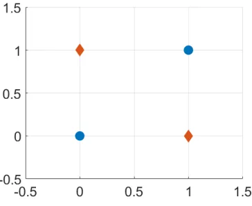
Figure 2.4 Binary example problem for NCA where blue circles and orange triangles define membership in the two classes: (a) original data, (b) 2-D mapping, (c) PCA mapping, (d) NCA mapping. . . 19

Figure 2.5 Neural network for the XOR example. . . 24

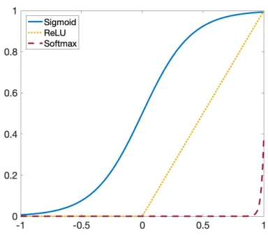
Figure 2.6 Common NN activation functions. . . 25

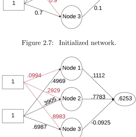
Figure 2.7 Initialized network. . . 26

Figure 2.8 Updated network after one full training iteration. . . 26

Figure 2.9 Final updated network after training. . . 27

Figure 2.10 Convolutional network structure. . . 28

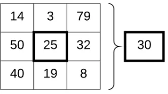
Figure 2.11 3_×3 mean pooling. The bold box in the center of the left indicates the pixel under consideration, the outer box indicates all the pixels pooled, and the bold box on the right hand side is the final result from the mean pooling. . . 29

Figure 4.1 Combine-then-classify workflow. . . 42

Figure 4.2 LOP (–) versus LgOP(- -) for two expert distributions (··) [42]. . . 47

Figure 5.1 17_×17 PWR assembly schematic. White indicates non-defect, gray in-dicates water channel/guide tube, red inin-dicates DCVD defect locations, and yellow indicates GET defect locations. . . 50

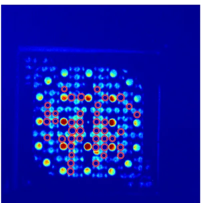
Figure 5.2 Hough transform applied to a DCVD image. . . 51

Figure 5.3 The first five principal components of (a) DCVD and (b) GET fuel rod sub-images. . . 54

Figure 5.4 DCVD fuel rod sub-image examples: (a) original defect, (b) reconstructed defect, (c) original non-defect, (d) reconstructed non-defect. . . 55

Figure 5.5 GET fuel rod sub-image examples: (a) original defect, (b) reconstructed defect, (c) original non-defect, and (d) reconstructed non-defect. . . 56

(13)

Figure 5.7 ROC Curve for each classification method under the combine-then-classify

scenario. . . 59

Figure 5.8 Classification results based only on DCVD data. . . 63

Figure 5.9 Classification results based only on GET data. . . 64

Figure 5.10 Classify-then-combine results for each classification methodology. . . 65

Figure 5.11 Combine-then-classify results for each classification methodology. . . 65

Figure 6.1 Example problem data with classes denoted by color. . . 74

Figure 6.2 Example problem, XYZ and RGB data sets. . . 75

Figure 6.3 Compression of DCVD data to 16 components for (a) NCA-mapped defect and (b) NCA-mapped non-defect; (c) Identity-mapped defect and (d) Identity-mapped non-defect; (e) mapped defect and (f) PCA-mapped non-defect. . . 77

Figure 6.4 Log scale eigenvalue plot for DCVD data. . . 78

Figure 6.5 Eigenvalues for ADCV D trained under with high burnup/short cooling time data with 36 overall defect (11 true defects) and 253 non-defects for 500 randomly sampledγ. . . 79

Figure 6.6 Compression of GET data to 16 components for (a) NCA-mapped de-fect and (b) NCA-mapped non-dede-fect; (c) Identity-mapped dede-fect and (d) Identity-mapped non-defect; (e) mapped defect and (f) PCA-mapped non-defect. . . 80

Figure 6.7 Log scale eigenvalue plot for GET data. . . 80

Figure 6.8 Eigenvalues for AGET trained under high burnup/short cooling time GET data with 36 defects and 253 non-defects for 500 randomly sampled γ. . . 81

Figure 6.9 Linear opinion pool weights for a 17×17 assembly using Euclidean norm distance metric for (a) DCVD and (b) GET. The weights for each fuel rod are directly mapped to [0,1] with the colormap axis for every rod location within the 17×17 grid. . . 83

Figure 6.10 Linear opinion pool weights for a 17_×17 assembly using Chebychev norm distance metric for (a) DCVD and (b) GET. The weights for each fuel rod are directly mapped with the colormap axis for every rod location within the 17_×17 grid. . . 84

Figure 6.11 γ densities after training for all 529 components of (a) DCVD and (b) GET. . . 85

Figure 6.12 Fuel rod sub-image for (a) non-standard guide tube 145 and (b) repre-sentative guide tube 91. . . 88

Figure 6.13 DCVD BNCAp(yi=def ect|xi) distribution means from Equation (6.1) for (a) TR1 and (b) Blind Test 1 with true defect in rod location 214. . . 88

Figure 6.14 DCVD BNCA MCMC random sampling chains for (a) Blind 1 defect and (b) representative Blind 1 non-defect. . . 89

Figure 6.15 GET BNCA p(yi = def ect|xi) distribution means from Equation (6.1) for (a) TR1 and (b) Blind Test 1 with true defect in rod location 214. . . 90

Figure 6.16 Means of estimated distributions for each TR1 fuel rod after training with (a) naive weighting, (b) Euclidean weighting, and (c) Chebychev weighting. . . 92 Figure 6.17 Estimated distribution means for Blind 1 with defect in rod index 214 for

(14)

Figure 6.18 Naive weighting MCMC chains for Blind Test 1 for (a) defect rod 214 and (b) non-defect rod 111. . . 94 Figure 6.19 Estimated p(yi = def ect|xi) for Blind 1: (a) defect rod 214, (b) guide

tube rod 91 and (c) non-defect rod 111. . . 95 Figure 6.20 Estimated distribution means for Blind 2 with defect in rod index 214 for

(a) naive weighting, (b) Euclidean weighting, and (c) Chebychev weighting 96 Figure C.1 Blind test 1 results for TR1 with (a) Naive weighting, (b) Euclidean

weighting and (c) Chebychev weighting. . . 117 Figure C.2 Blind test 2 results for TR1 with (a) Naive weighting, (b) Euclidean

weighting and (c) Chebychev weighting. . . 119 Figure C.9 Blind test 1 results for TR1 with (a) naive weighting, (b) Euclidean

weighting and (c) Chebychev weighting. . . 122 Figure C.15 Blind test 7 results for TR1 for (a) Naive weighting, (b) Euclidean

weighting and (c) Chebychev weighting. . . 122 Figure C.17 Blind test 1 results for TR1 for (a) naive weighting, (b) Euclidean

weight-ing and (c) Chebychev weightweight-ing. . . 123 Figure C.18 Blind test 2 results for TR1 for (a) Naive weighting, (b) Euclidean

(15)

Figure C.21 Blind test 5 results for TR1 for (a) Naive weighting, (b) Euclidean weighting and (c) Chebychev weighting. . . 124 Figure C.22 Blind test 6 results for TR1 for (a) Naive weighting, (b) Euclidean

weighting and (c) Chebychev weighting. . . 125 Figure C.25 Blind test 1 results for TR1 for (a) naive weighting, (b) Euclidean

weight-ing and (c) Chebychev weightweight-ing. . . 126 Figure C.26 Blind test 2 results for TR1 for (a) Naive weighting, (b) Euclidean

(16)

Chapter 1

Introduction

1.1 Problem Statement and Application

The International Atomic Energy Agency (IAEA) is the international governing body for nuclear facilities, technology, and agreements. Although established in 1957, it was the 1970 Nonprolif-eration Treaty (NPT) that made the IAEA an integral part of nuclear facilities and opNonprolif-erations across the world [29]. IAEA inspectors visit facilities around the world to conduct inspections and ensure the use of nuclear technology for peaceful purposes. One particular aspect of in-spection, spent fuel monitoring, has been a pillar of safeguards agreements for several decades. One of the first Comprehensive Safeguards Agreements (CSA) between the IAEA and Canada, completed in 1972, includes required material accounting of spent fuel in storage [3]. At nu-clear plants, spent fuel is stored in wet storage (cooling ponds) until it cools. It can then be transferred to dry storage in concrete casks or sent to permanent storage facilities. In France and Japan, spent fuel is reprocessed for future use in nuclear facilities. The primary motiva-tion for spent fuel inspecmotiva-tions is material accounting–the host country must be able to show where all potentially weapons-usable material is at a given time in order to confirm its usage for exclusively peaceful applications.

There are two kinds of defects that inspectors look for in spent fuel assemblies: gross defects, where an entire fuel assembly is a non-fuel item, or partial defects, where≥50% of the individual fuel rods in an assembly are non-fuel items. These non-fuel items cover both cases where the fuel item has been completely removed and cases where the fuel item was replaced with a non-fuel item, such as steel. Ideally, the IAEA would like to identify when even a single fuel rod within an assembly is a non-fuel item.

(17)

Figure 1.1: Spent fuel cooling pond [1].

of data taken during these measurements.

In particular, the Digital Cerenkov Viewing Device (DCVD), described in Section 1.2.1, has been used since the mid 1980s as a gross defect detection technique. In more recent years, gamma emission tomography (GET), in Section 1.2.1, has emerged with the potential for use as a single rod defect detection method. Past research has shown that for large assemblies–for example, a standard 17×17 assembly– and in varying burnup and cooling time scenarios, both DCVD and GET have weaknesses when determining defects. Whereas DCVD remains a gross defect method, it is a much cheaper option than GET which, as currently implemented, requires several detectors placed at multiple heights along an assembly for high accuracy.

The goal of our investigation is to combine the complementary strengths and weaknesses of DCVD and GET spent fuel measurement methods to develop a robust single fuel rod defect detection method. Using GET data from only a single height along a given assembly and DCVD data that provides a top-down view of that same assembly, we will incorporate the best of both methods while minimizing their weaknesses for a more robust and automated identification of defects in spent fuel ponds.

(18)

gen-Figure 1.2: Pressurized Water Reactor (PWR) schematic [51].

erate comprehensive libraries. Additionally, the robust combination of data through Bayesian fusion methods will be unique in its nuclear safeguards application. Finally, the combination of Bayesian Neighborhood Component Analysis (BNCA) with Bayesian data fusion provides a unique and new mathematical formulation addressing the combination of data from varing detectors and of varying sizes in a supervised learning context.

1.2 Background and Prior Work

1.2.1 Nuclear engineering methods and background

There are two primary classes of nuclear reactors currently in operation: boiling water reactors (BWRs) and pressurized water reactors (PWRs). PWRs are the focus of this work, with a general schematic as shown in Figure 1.2. In that schematic, the fuel is shown as individual fuel rods. In fact, the fuel is an array orassembly of rods, with arrays varying in size. In our data set, we consider 17×17 PWR fuel assemblies shown in Figure 1.3. Thus, there is a consistent general geometry of the assembly, and each fuel rod in an assembly is numbered according to the pin map depicted in Figure 1.4. Once the fuel assemblies are removed from the reactor, they are stored in cooling ponds, as depicted in 1.1. The spent fuel, once in storage in cooling ponds, is the focus of our research.

(19)

Figure 1.3: 17×17 PWR fuel schematic [15].

detected by spent fuel inspection tools.

Digital Cerenkov Viewing Device (DCVD)

Cerenkov light is light produced in the visible spectrum by charged particles moving faster than the speed of light in a given medium. The Digital Cerenkov Viewing Device (DCVD) is a specialized, stationary camera used to photograph the Cerenkov radiation emitted from spent fuel rods in wet storage; see Figure 1.5. Another version of this detector is the Improved Cerenkov Viewing Device (ICVD) [30], which, for simplicity, can be considered the video version of the DCVD. DCVDs are currently widely implemented in IAEA inspection sites but the handheld ICVDs are becoming more common in inspections [30]. Renewed interest in DCVDs to inspect large quantities of spent fuel before relocation to long-term storage motivates our focus on this method [9]. Additionally, the data gathered from ICVDs are videos that can be split into frames, so the analysis performed on still images remains applicable.

(20)

Figure 1.4: 17_×17 Pin map: gray = fuel rod, white = guide tube, yellow = DCVD defect location, red = GET defect location [49].

middle of the camera, and loses sensitivity moving towards the edge of the field of view due to collimation effects.

The Applied Nuclear Physics group at Uppsala University and their collaborators have been very influential in both the CVD and GET development. This group has worked on simulations, and various improvements of those simulations, for DCVD images [8], as well as template matching in the resulting image [9]. Within the scope of the simulations, they have also investigated various properties of spent fuel that impact the simulations and how to adjust for those impacts. Additionally, they have produced recommendations for improving the DCVD data collection process [9].

(21)

Figure 1.5: Digital Cerenkov Viewing Device (DCVD) [12].

The speed of measurement of DCVD, at 10-30 seconds per assembly, constitutes a significant advantage of the method [7]. Additionally, DCVD is accurate specifically in low burnup and long cooling time scenarios, where many other detection methods are more limited. Finally, the 15% removed/substituted requirement for accurate defect detection is heavily impacted by assembly hardware. Whereas assembly hardware cannot be modified, even a small amount of extra information from a detection method not limited by hardware and DCVDs other drawbacks could provide a large increase in defect detection accuracy.

(a) (b) (c)

(22)

Gamma Emission Tomography (GET)

Another method currently under investigation as a single defect detection method for safe-guards implementation is gamma emission tomography (GET), a prototype of which is shown in Figure 1.7 [52]. In this method, the detector is a collar that encircles a fuel assembly, taking measurements at a particular height along the assembly. This collar detector setup permits in-creased accuracy in defect detection around the outer edges of the assembly [49]. However, this same setup requires either that the detector be submerged near highly radioactive material, shortening the equipment lifetime, or a time- and labor-intensive process of moving the fuel assembly from the cooling pond to a hot cell for inspection. In addition, the GET measure-ment time is an order of magnitude larger than that of DCVD–hours rather than seconds for a measurement [49]. This makes the GET method significantly more expensive than DCVD. Finally, GET detection methods rely on the ability of emitted gammas to reach the detector without being absorbed within the assembly. However, in the larger pressurized water reactor (PWR) fuel assemblies, GET demonstrates limited sensitivity due to the large size of the as-sembly and small inter-rod distances [49]. For PWR fuel, depending on burnup and cooling time scenarios as well as where a defect is located within an assembly, GET has between a 20% and 95% probability of identifying a single defect [49]. The 95% probability is limited to high burnup/short cooling time scenarios [49]. For low burnup and long cooling times, GET has a 20-25% probability of identifying a single defect with a false positive rate at 10% [49]. Note that these rates are with simulated data with 20% rod-to-rod variation, but otherwise ideal measurement scenarios.

The GET data in this work comes from Pacific Northwest National Laboratory PNNL); for detailed simulation parameters, see [49]. Sinograms were simulated with Monte Carlo N-Particle Transport Code (MCNP) by calculating sinograms for single pins, summing them, and adding Poisson noise to account for pin-to-pin variation. The integration time, 3.89 seconds, is consistent with a one hour measurement. Reconstructions were then calculated using a filtered back projection algorithm. Sinograms and reconstructions for the data used in this work are plotted in Figure 1.8. There are two cases of burnup and cooling times considered in this work, and both are shown in Figure 1.8. Case 1 is a high burnup, short cooling time scenario, and Case 2 is a low burnup, long cooling time scenario. For details, see Table 5.1.

Gamma emission tomography has been a field of interest for many years, and has been difficult to perfect. Experimental information [31, 34] and simulated data [32, 33, 49, 50, 57] have both been produced through the years. Similar to DCVD research, prior related work has focused on template matching and fuel rod location identification [14]. Current tomography research has focused on multiple methods of cross-section recreation, but the data provided by Pacific Northwest National Laboratory and used for this investigation implements filtered back projection [49].

(23)

Figure 1.7: Gamma Emission Tomographer (GET) [16].

removal and substitution, whereas DCVD is primarily limited to removals. In the larger PWR assemblies, and in low burnup/long cooling time scenarios, the single defect detection is about 25%. The major drawback of GET is the cost and time required; a standard measurement takes an hour as opposed to DCVD’s 30 seconds. Additionally, the GET detector has to be submerged with the assembly in the cooling pond or the assembly removed from the cooling pond into a hot cell. Finally, the GET detector also requires multiple detectors at multiple heights along the assembly for best accuracy.

The goal of our research is to investigate defect detection accuracy when DCVD measure-ments are combined with GET measuremeasure-ments taken at only a single height along the assembly.

1.3 Outline and Significant Contributions

In this dissertation, we discuss the methods we developed and implemented to solve the problem of defect detection using both DCVD and GET data. In Chapter 2, we discuss machine learning methods and their strengths and weaknesses, specifically in the defect detection problem. In Chapter 3, we discuss various optimization algorithms typically implemented in the training of machine learning algorithms from Chapter 2. The mathematical concepts of data fusion are introduced in Chapter 4, followed by non-Bayesian classification results in Chapter 5. Finally, Chapter 6 presents a novel pipeline algorithm that combines Bayesian classification and data fusion for probabilistic classifications.

(24)

(a) (b) (c) (d)

(e) (f) (g) (h)

Figure 1.8: Tomographic reconstruction data set [49]: (a) Case 1, Image 1, (b) Case 1, Image 2, (c) Case 2, Image 1, (d) Case 2, Image 2, (e) Case 1, Sinogram 1, (f) Case 1, Sinogram 2, (g) Case 2, Sinogram 1, (h) Case 2, Sinogram 2.

In Chapter 6, we present Bayesian classification results. In particular, our contributions focus on compression, fusion, and again, our spent fuel application. Our proposed compression technique, using Cholesky factors within the BNCA framework, maintains the Mahalanobis na-ture of our learned metric, whereas the original BNCA formulation in [54] does not. The second main contribution in this chapter is the development of a fusion pipeline, the BNCA+LOP Pipeline algorithm, built around the BNCA algorithm. This pipeline aggregates data from multiple sources of differing sizes and quality, providing probabilistic classifications as output.

(25)

Chapter 2

Machine Learning Overview

2.1 Machine Learning Methods

To develop the machine learning methods used throughout this work, we start with a motivating example: the exclusive or function (XOR) [21]. The data points are shown in Table 2.1, with true and false as the classes (denoted by 1 and 0 respectively). From a plot of this data in Figure 2.1, we can see that the classes are notlinearly separable; i.e., we cannot draw a single line between the two classes to separate them. Because the data is not linearly separable, we cannot easily separate the data into two classes and hence we need classification methods that don’t rely on linearity.

The following sections detail several methods for solving this problem with machine learn-ing. We detail the associated optimization methods in Chapter 3, including gradient descent, stochastic, and Newton’s method-based algorithms.

2.1.1 Supervised versus Unsupervised Learning

There are two broad classes of machine learning algorithms: supervised and unsupervised algo-rithms. Supervised learning takes advantage of anylabels that may come with the original data for which we’re learning a classification algorithm. For example, in the XOR problem, the labels are the true and false categorizations of each data point. Supervised methods use these labels by penalizing incorrect classifications during the training stage for a final trained algorithm that

Table 2.1: XOR data points with true and false denoted by 1 and 0, respectively.

x1 x2 Class Graph legend

1 1 0

0 0 0

0 1 1

(26)

Figure 2.1: XOR graph.

best fits both the original data and their known labels. In the case of our nuclear application, the labels are defect/non-defect, or when extended beyond the simple binary problem, defect, water tube/guide channel, and present rod.

If the XOR example did not have any true/false labeling, then we would employ unsuper-vised learning. In unsuperunsuper-vised methods, there are no true labels by which we can penalize an incorrect classification. Instead, unsupervised methods rely on identifying some structure within the data based on similarities and differences between points according to a variety of heuris-tics. Generally, because there is no associated ground truth that the algorithm can compare its performance against, unsupervised methods require more data than supervised methods to be able to identify classes in a data set.

2.1.2 k-Nearest Neighbors

Intuitively, it makes sense to classify a data point based on the class of its neighbors; this is the principle behind k-Nearest Neighbors (kNN). We denote our data set as X, with the columns as the individual data vectors, x. Let k indicate the number of neighbors used to classify a particularx, andd(x,y) be the distance between two pointsxandyin our set given some distance metric. Given a point x, the kNN algorithm searches through all points in the data matrix X until it finds the k points closest to the point x based on a distance metric

d(x,y). In the kNN context, both the number of neighbors k and the distance metric d(·,·) are parameters that can be learned during a training stage. We provide an overview of the algorithm in Algorithm 1.

With the XOR example, we consider the pointx= (1,1)T_{. Our goal is to determine whether}

(27)

Algorithm 1:kNN Algorithm from [4]

Result: kNN classification of data

Initialization: choose number of neighbors kand metric d;

for allxi data points in our set do

Calculated(xi, xj) for allj

Selectxk_ij as thekvalues of xj that maximize d(xi, xj) for each xi

switch do

To fit a new model:return the mean of the neighborhood labels to classifyxi

To classify with an existing model:return the mode of the neighborhood labels to classify query point xi

end end

neighbors, given a Euclidean distance metric with

d(x,y) =

N X

i=1

(xi−yi)2 !1₂

,

we would classify the pointx= (1,1)T _{as belonging to class 1.}

Because we know that the true label of the point x = (1,1)T _{is in fact 0, clearly kNN}

with our choice of parameters is not the best classifier for this problem. In fact, there is no set of parameters using kNN on its own for this problem that will correctly classify the point

x= (1,1)T_{. Another issue with kNN is the following. Had we chosen only one nearest neighbor,}

this Euclidean distance metric would have yielded a tie between the two nearest points as they are each equidistant tox. Ties can be addressed by the implementation of a tie-breaking criteria [4]. Examples of tie-breakers include randomly choosing between the tied points or simply choosing the point that appears first in the data set.

Another issue that may arise, but which we don’t see in the XOR problem, is if there is no clear classification among the neighbors. In the case of two nearest neighbors, this manifests as both neighbors belonging to a different class, which raises the question of how the new point is classified. This can be solved by either increasing or decreasing k until the tie is broken, or weighting the neighbors under consideration inversely proportional to their distance from the point being classified [4].

(28)

Figure 2.2: Two nearest neighbors, Euclidean distance.

2.1.3 Principal Component Analysis

In principal component analysis (PCA), the goal is to remap data to a new space that maximizes the variance in a data set [5]. In theory, maximizing the variance will permit identification of any trends in the data and improve the ability to separate classes.

Let_{xn}Nn=1denote a set ofNobservations, where eachxnis aD-dimensional column vector.

The idea of compression with principal component analysis is to project the data_{xn}Nn=1 from

its initial D dimensions to a space with dimensionality M << D [5]. The sample covariance matrix of the data in the original D-dimensional space is defined to be

S= 1

N ₋1

N X

n=1

(xn−¯x)(xn−¯x)T.

For an introduction to the mathematics of PCA, we assume for now that M = 1, so we are projecting our data onto a 1-dimensional space [5]. The goal of PCA is to identify the mapping such that the variance in the new 1-dimensional space is maximized. Let this new 1-dimensional subspace be defined by some vector u1; if the data set variance in u1-space is

maximized, it is the first principal component. For now, assume that ||u1||= 1, as a non-unit norm would appear only as a coefficient carried through this derivation. Each data point in {xn}is projected into the space defined by u1 and can be expressed asu1Txi fori∈1, . . . , M.

The variance of the projected data is uT₁Su1 [5], where S is the covariance matrix defined in the originalD-dimensional space andx¯ is the sample average of the data set,

¯ x= 1

N

N X

n=1 xn.

(29)

u1, constrained so||u1||stays finite. We thus have a constrained optimization problem with a

Lagrange multiplier,uT₁Su1+λ1(1−uT1u1). Taking the gradient with respect tou1 and setting

it equal to 0, we find that uT

1Su1 = λ1, implying that u1 must be an eigenvector of S with

the associated eigenvalue λ1. The variance is maximized when u1 is the eigenvector with the

largest eigenvalueλ1 [5]. Thus, vector u1 is the first principal component.

The process continues similarly for any subsequent principal components u2,u3, . . . ,uM

when M >1, with the constraint that each component is orthogonal to all the prior principal components. The final set of components is an orthogonal basis for the new space onto which the data is projected. This orthogonalization can be done via the standard Gram-Schmidt algorithm; see [56] for details, or, if data is centered, via singular value decomposition (SVD) as detailed later. When all the principal components have been defined, we can reconstruct the original data via the relation

x_≈x¯+

M X

i=1

xT_nui−x¯Tui

ui. (2.1)

If the data is centered; i.e., the mean is subtracted from all data vectors, then we can solve the eigenvalue/eigenvector problem using singular value decomposition (SVD) [53]. When the data is centered, the sampled covariance matrix S is S = _N1₋₁XTX, where X is the N ×D

data matrix with N observations of D variables. The covariance matrix is nonnegative and symmetric. Hence it is diagonalizable, and can be expressedS=VLVT,whereVis the matrix of eigenvectors ofS–and ofXT_X_{by our covariance definition in the centered case–and}_L_{is the}

diagonal matrix of eigenvalues of S [53]. This aligns with the previous derivation of principal components as eigenvectors of S. However, if we take the singular value decomposition (SVD) of our original data matrix, we obtain

X=UΣVT,

where U is unitary, Σis the diagonal matrix of singular values, and V is the matrix of eigen-vectors ofXTX [53]. The covariance matrix is now

S= 1

N−1VΣ

T_UT_UΣVT_. _(2.2)

Because U is unitary, UTU = I. The matrix Σ is diagonal so Σ2 is comprised of squared singular values along its diagonal. Equating our two definitions forS,we obtain

S=VLVT = 1

N −1VΣ 2_VT_.

(30)

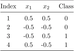
Table 2.2: Centered XOR data points.

Index x1 x2 Class

1 0.5 0.5 0

2 -0.5 -0.5 0

3 -0.5 0.5 1

4 0.5 -0.5 1

computed using an SVD of the original data.

In the XOR example, centering the data yields the points in Table 2.2. Since the data is cen-tered, we can compute the principal component mapping using singular value decomposition. Often, compression is required due to computational limitations. However, we may be able to compress data by examining the decay of the eigenvalues. If there is a significant gap in eigen-value magnitude, or if they fall below a user-defined threshold, then the principal components will be all components corresponding to eigenvalues above this magnitude change/threshold. In this particular case, we have no compression, and the principal components of the centered data are simply the standard R2 basis, [1,0] and [0,1]. In this particular case, PCA does not change the current data mapping. This implies that the variance within our data is already maximized.

This example shows an important flaw of PCA for classification; maximizing the data vari-ance does not imply that we have maximized the number of correct classifications. When a data set is unlabeled; i.e., we don’t know the true classifications of any data points, maximizing the variance is often the best choice. In this case, PCA can identify patterns inherent in the data without requiring extra information. However, if we have labeled data, we would like to see a classifier maximize the number of correct classifications. This corresponds to a change in objective function, encapsulated by Neighborhood Component Analysis.

2.1.4 Neighborhood Component Analysis

Neighborhood Component Analysis (NCA) [22] is a supervised version of PCA. The principle is to construct a mapping into a space where the classifier of choice for a problem performs optimally on a labelled data set. PCA maximizes the variance within a data set and remaps to a space where that variation is best separated; NCA instead attempts to learn a mapping into a space where we maximize the number of correct classifications in a data set. To accomplish this, the classifications of the data must be known, thus making this a supervised learning method. Data is classified by mapping a new data point using a Mahalanobis matrix transformation

(31)

between two pointsx andy such that

d(x,y) = q

(x−y)T_Q₍_x₋_y₎_.

Here Q is a symmetric non-negative definite matrix; i.e., Q = ATA for some A [48, 59]. In the NCA context, this metric measures the dissimilarity between two points belonging to the same class. Because of the definition of Q, NCA functionally learns a distance metric

d(x,y) = (Ax₋Ay)T₍_Ax₋_Ay_{) [22]. This}_A _{matrix is what we employ in the definitions of}

NCA and its variants.

We define our data set as {xi}Ni=1, where N is the number of observations, and each xi

has a corresponding classification Ci, such as True/False or 0/1 in the XOR example. NCA

maximizes the function

J(A) =

N X

i

pi= N X

i X

j∈Ci

pij, (2.3)

where the value pij is defined by

pij =

exp _−||Axi−Axj||22

P k6=i

exp −||Axi−Axk||22

. (2.4)

The value of pij can be interpreted as the probability that pointxi will be classified using the

point xj. The sum pi is the sum over the probability that point xj is used to classify pointxi

for all xj in the same class as xi; i.e., is the total probability that a neighbor in the correct

class is used to classify xi. The value of pi is always between zero and one, indicating that it

is, indeed, a valid probability measure [22]. Then the total over all pi is J(A), the number of

points classified correctly across the data set. The gradient, _∂∂J_A,is

∂J ∂A = 2A

X

i 

p_i X

k

pikxikxTik− X

j∈Ci

pijxijxTij 

, (2.5)

wherexij =xi−xj.

Thepij function is relatively smooth and both the function and derivative are defined almost

everywhere. The cost functional J(A) can thus be optimized using gradient descent methods with the analytic gradient in Equation (2.5) or with other optimization routines detailed in Chapter 3.

After A is computed via optimization methods using a set of training points, a new point can be classified by using the learned A to map into the transformed space, and subsequently using kNN in the A-space to compare it with previously classified points.

(32)

data set, and neighborhoods for each point are recalculated at each step. This adds significant computational expense with limited ability to parallelize the algorithm.

Using the example XOR problem, we start by calculating the pij values for each of the four

points. In the NCA case, we consider all neighbors of a given point when calculating the pij

values with Equation (2.4). To give a consistent comparison with the PCA example, we again center the data, although this is not required in NCA. We then have the data shown in Table 2.2. Centering does not affect the classifications.

For a simple example, let A be the identity for our first step, so we can use the points directly to calculate all relevant parts. Using NCA definitions, we calculate alld2_ij values,

d2₁₂=_||x1−x2||22= 2,

d2₁₃=_||x1−x3||22= 1,

d2₁₄=_||x1−x4||22= 1,

where the bold face indicates the vector xi = (x1, x2)i with index i. Once we have computed

all d2

ij values, we can calculate all pij values. Again, we show only those for i= 1 for brevity

and note that

p12=

exp(₋d2₁₂) P

k6=i

exp(−d2_ik) =

exp(₋2)

exp(−2) + exp(−1) + exp(−1) = 0.1554,

p13=

exp(−d2 13)

P k6=i

exp(₋d2_ik) =

exp(−1)

exp(−2) + exp(−1) + exp(−1) = 0.4223,

p14=

exp(−d2₁₄) P

k6=i

exp(₋d2

ik)

= exp(−1)

exp(₋2) + exp(₋1) + exp(₋1) = 0.4223.

The values ofpi are then

p1 = 0.1554,

p2 = 0.1554,

p3 = 0.1554,

p4 = 0.1554.

Because of the symmetry in our original problem, all are equal at this first step. Here J(A) = 4×0.1554 = 0.6216. In the NCA formulation, thisJ(A) quantity is the number of points that choose a point in their same class as a neighbor, or equivalently, the number of points that are classified correctly. Calculating the gradient, gforA as the identity yields

g(A) = "

−0.525 0 0 ₋0.525

#

(33)

(a) (b)

Figure 2.3: Final optimization mapping for two different initial guesses: (a) A0 = identity matrix and (b)A0 = PCA of the original data.

The step will vary based on the employed optimization method but, for simplicity, we employ steepest descent for this example, with λ = 1. For more information on steepest descent and other optimization routines, see Chapter 3. Our new matrix is then

Ai+1 =Ai− ∇J(Ai)

= "

1.525 0 0 1.525

#

,

and we evaluate J(Ai+1) and J(Ai+1) again to determine the next step. Eventually, we will

arrive at someA∗whereJ(A) is maximized. We note that NCA is very sensitive to initial values as demonstrated by the results shown in Figure 2.3. The A∗ that maximizes J(A) for initial value of the identity is scaled down, but is otherwise the same as the original XOR mapping. TheA∗ mapping from an initial value of all ones, however, maps both [0,1]T _{and [1}_,_0]T _{to the}

origin while keeping the other two points further away. These are clearly two very different final mappings and it is unclear which to choose as the final A∗ choice. With A0 as the identity,

NCA performs no better than PCA. WithA0 as the matrix of all ones, the final mapping sends

the two points with class 0 both to the origin, marginally improving our overall classification result as compared with PCA. This dependence on initial values remains a problem wherever this method is employed. Two common starting points are either the standard Rk basis for a

k−dimensional subspace, or the PCA mapping of the data into ak−dimensional subspace. We illustrate a different and more complex example problem in Figure 2.4 to demonstrate the power of NCA when separating larger data sets [17]. The goal is to map a 3-D set of data to 2-D. The original 3-D data is comprised of 300 points belonging to two different classes. The

(34)

(a) (b) (c) (d)

Figure 2.4: Binary example problem for NCA where blue circles and orange triangles define membership in the two classes: (a) original data, (b) 2-D mapping, (c) PCA mapping, (d) NCA mapping.

within this example, they are notably not the same mapping. The scale of the NCA mapping is much different than that of PCA, it separates the two classes without overlap, and the data in the transformed space is linearly separable. The PCA mapping separates the classes, but there is still some minor overlap in the middle, and the data is still not linearly separable. This is not to say that NCA will always find a mapping that is linearly separable; however, the difference in objective function between PCA and NCA leads to noticeably improved classification here. In classification problems, therefore, the NCA-learned mapping is often the better choice when data labels are available.

2.1.5 Fast Neighborhood Component Analysis

The major difference between Fast Neighborhood Component Analysis (FNCA) [60] and tradi-tional NCA is a restriction in the neighbors considered within the calculation of eachpiandpij.

This enables computational speedup in the algorithm without sacrificing the NCA framework. The value pij is now calculated as

pij =

exp(_−||Axi−Axj||2)

P k∈MiSHi

exp(−||Axi−Axk||2)

,

where Mi is the set of k neighbors in the same class as point xi and Hi is the set of k nearest

neighbors in all other classes. The definition for pi is also changed by this formulation and is

now

pi = X

j∈Mi

pij.

(35)

In the simple 300 point classification problem from Figure 2.4, this minor change in formu-lation, and the similar change in pi’s definition to sum over only the j ∈Mi, yielded a nearly

3-fold decrease in timing. On our sample problem with 300 3-dimensional points, it went from a 230 second optimization using traditional NCA to an 80 second optimization.

2.1.6 Bayesian Neighborhood Component Analysis

Bayesian Neighborhood Component Analysis (BNCA) [54] is formulated similarly to the original NCA, with the same distance definition. However, in BNCA, the goal is to learn a distribution corresponding to the mapping A. By doing so, the BNCA framework enables the estimation not only of a new point’s classification, but also the associated distribution.

The objective function to be maximized is now a posterior estimation distribution,

J(A) =Y

i

P(Y|X,A)p(A), (2.6)

where P(Y|X,A) is the likelihood and p(A) is the prior distribution. The prior incorporates any pre-existing knowledge about our data set, whereas the likelihood is the probability of a variable taking a certain value given observed data.

To perform this maximization, we need a formulation for each term within this objective function. BNCA learns an A under a set of assumptions that permits estimation of both the prior and likelihood, and thus the posterior. Note that this method will still achieve the same goal as NCA and FNCA; we’re still maximizing the probability that a point xi is closer to a

point in its same class after transformation by the matrix A. In the BNCA case, however, we are additionally fitting a distribution to the class memberships, providing probabilistic classifi-cations for each data point.

To reformulate this problem in the already established NCA framework, define

P(yi=k|xi,YNi,XNi,A) =

P j∈Ni

1{yj =k}exp(−d2_Aij)

P t∈Ni

exp(₋d2

Aij)

,

where{yi=k} is the equivalence function defined by

{yi=k}= (

1, yi = Class(xi) =k,

0, otherwise

and the distance d_Aij is defined by

d2_Aij = (xi−xj)TA(xi−xj).

(36)

original NCA formulation, whereQ is symmetric positive semi-definite. The likelihood is then

P(Y_|X,A) = 1

Z(A) Y

i

P(yi|xi,YNi,XNi,A),

whereZ(A) is a normalizing constant.

As in NCA, the principle is to learn a Mahalanobis metric to maximize the number of points classified correctly, while estimating the associated distributions. The BNCA approach starts by approximating the matrix A as a linear combination of the eigenvectors of the data in a manner similar to PCA.

We define this approximation as

A=

b X

`=1

γ`v`v`T,

where v` the `th eigenvector of our data matrix XXT, γl are the coefficients in the linear

combination, and b denotes the number of eigenvectors used in the approximation. Note that γ is a column vector ofγ` values, but eachv` is a column vector. Our probability can then be

expressed as

P(yi=k|xi,YNi,XNi,A) =

P j∈Ni

1_{yj =k}exp

−(xi−xj)T b P `=1

γ`v`vT`(xi−xj)

P t∈Ni

exp

−(xi−xt)T b P `=1

γ`v`vT_`(xi−xt)

(2.7)

= P j∈Ni

1{yj =k}exp

−d2_γij

P t∈Ni

exp₋d2_γit

(2.8)

=P(yi =k|xi,YNi,XNi,γ). (2.9)

Here we define d2_γij = d2_Aij =γTwij with γ = [γ1, . . . , γb]T, w`ij = (v`T(xi−xj))2, and wij =

[w_ij1, . . . , w_ijb]T_{. The distance function is now denoted} _d2

γij for any points xi,xj, though this is purely notational and designed to indicate that we are estimating γ rather thanA directly.

To compute the posterior distribution of A, we need only compute the posterior distribu-tion for γ. Assume that p(γ) = N(γ_|m0,V0); i.e., that γ is normally distributed with mean

(37)

all N data points and allK classes, the log-likelihood,`, is then L= N X i K X k

1_{yi=k}log{p(yi=k|xi,YNi,XNi,γ)}.

The summations take all points and classes into account, while_{yi=k}term ensures the inner

sum over possible classes only considers one class designationk at a time.

Employing the definition of p(yi =k|xi,YNi,XNi,γ) and using the fact that log(a+b) >

log(a) + log(b) if 0< a, b <1,we obtain

L >X

i X

k

1_{yi=k} 

 X

j∈Ni

log_{yj =k}exp

−d2_γij

−logX

t∈Ni

expd2_γit

  >X i X

j∈Ni

yijlog 

 

exp(−d2

γij)

P t∈Ni

exp(−d2_γit)

   >X i X

j∈Ni

yijlog 

 

1 1 + P

t∈Ni

exp(d2

γij−d2_γit)



 .

We then employ the definition of the log-sum-exp function, lse(ηij) = log 1 + P t∈Ni

exp(η_ijt) !

, where we define ηt_ij = (wij −wit)Tγ. It follows that

L >₋X

i X

j∈Ni

yijlse(ηij),

whereyij =δij is the Kronecker delta [54].

Bohning’s quadratic bound [6] applied to thelse function yields

lse(η)_≤ 1 2η

T_A_η₋_bT

ψη+cψ,

where

A= 1 2(IM −

1

M + 11M1

T M),

bψ =Aψ−g(ψ),

cψ =

1 2ψ

T_Aψ₋_g₍_ψ₎T_ψ₊_lse₍_ψ₎_.

Here M indicates the size of our matrices. LetNiκ denote theκ

th_{nearest neighbor of point}_x

i, and letψij be the variational parameter

(38)

L >X

i X

j∈Ni

yij

−1 2γ

T_Wj iH(W

j i)

T_γ₊_bT ij(W

j i)

T_γ₋_c ij

,

where

W_ij = [wij −wiNi₁, . . . ,wij−wiNiκ],

H= 1 2

Iκ−

1

κ+ 11κ1

T κ

,

bij =Hψij −g(ψij),

g(ψij) = exp(ψij −lse(ψij)).

Herecij is a constant,κ is the number of nearest neighbors,Iκ is the identity of sizeκ×κ, and

1κ is a lengthκ vector of ones.

Using the prior distribution N(γ|m0,V0) and the likelihood estimate lower bound from the Bohning’s quadratic bound step, we can directly compute the posterior distribution of γ,

N(γ_|mT,VT) where

VT = 

V₀−1+ X

i X

j∈Ni

yijWijH(W j i) T   −1

mT =VT 

V

−1 0 m0+

X

i X

j∈Ni

yijW_ijbij 

.

The variational parameter is updated by the computation

ψij = (W_ij)TmT. (2.10)

This update process is repeated to self-consistency.

The prediction for a new point xi can be found with the estimation of p(yi|xi,YNi,X)

using Markov Chain Monte Carlo (MCMC) methods, summarized in Appendix A, such that the continuous distribution is approximated by

p(yi|xi,YNi,XNi) =

Z

γ

p(yi|xi,YNi,XNi,γ)q(γ)dγ≈

1

T

T X

t=1

p(yi|xi,YNi,XNi, γt).

Here γt is a set of T points sampled from our constructed Gaussian distribution of q(γ) = N(γ|mT,VT) that approximates the continuous distribution. Note that whereas q(γ) is a

Gaussian, p(yi|xi,YNi,XNi,γ) is a multivariate normal distribution.

There is some capability to incorporate the FNCA speedup in the restriction of the neigh-borhoods Ni in the calculation of pij throughout the BNCA framework. The Ni restriction

(39)

Figure 2.5: Neural network for the XOR example.

point xi, the corresponding calculation of pi is limited to looking at points in a user-defined

neighborhood.

2.1.7 Neural Networks

Neural networks (NN) can be motivated with our exclusive or (XOR) problem. A neural network does not require data to be linearly separable, making it ideal for this problem.

Consider the network depicted in Figure 2.5, comprised of 2 input nodes, one hidden layer with three nodes, and one output node. The input is one of the four possible combinations of

x1 and x2, and the output is in the interval [0,1]. For a layer`, the weight at node j acting on

output from nodekis denoted byw_jk` .In this network,`= 1,2 and 3. The input is layer `= 1, the hidden layer is `= 2 and the output is`= 3. The weights are indexed accordingly.

The final output of the network can be expressed as

y=σ

w₁₁3 σ i1w112 +i2w122

+w3₁₂σ i1w221+i2w222

+w3₁₃σ i1w231+i2w322

, (2.11)

where i denotes the inputs component, σ denotes an activation function, and w denotes the weights, all as indexed in the image. In this example, we take the activation function to be the sigmoid function,

σ(vi) =

1

1 +e−vi. (2.12)

Other choices include the the Rectified Linear Unit (ReLU),

σ(vi) = max(0, vi) (2.13)

and the softmax function,

σ(vi) =

evi

P k=1

evk, (2.14)

(40)

Figure 2.6: Common NN activation functions.

favoring 0 or 1 rather then the values in between, so we use the sigmoid function bounded to the [0,1] interval.

The randomly initialized network for the XOR example is shown in Figure 2.7 with the input (1,1), and the output calculated with Equation (2.11) is 0.6785. Because our data set is labeled, we know the output should be 0, making the error e=d−y= 0.6785,where dis the target output and y is the network output.

For simplicity, we demonstrate here a gradient descent update where the objective function to minimize is thee=d−y function, withyas the network output andddefined as the target output. We provide a detailed discussion of gradient descent and other optimization methods in Chapter 3.

The weight update for gradient descent defines the update such that

wi+1=wi+λ∇ewi,

whereewi is the function e=d−y evaluated with the weightwi.

Back propagation, covered in Section 2.2, is the process of propagating the error e back through the network so that the weight update can be defined for every node and weight in the network. Here, we implement the process outlined in Section 2.2 with a gradient descent step with objective function e= d₋y. A single step yields the weights shown in Figure 2.8. The final trained network is shown in Figure 2.9.

(41)

For all considered binary classification, the cross-entropy cost functional,

J =

M X

i=1

[₋diln(yi)−(1−di) ln(1−yi)], (2.15)

where M is the number of training vectors, replaces e when more than one training vector is present. Network weights are updated via back-propagation of this error until the performance reaches a desired goal; i.e., cost functional is minimized. Chapter 3 provides other cost functional examples as well as other optimization updates.

Note that this network has been trained only on the point (1,1), and has learned that classification very well, with an output of 3.5_×10−4 _{instead of the initial value of 0.6785.}

However, if we test the other XOR points with this network, we obtain outputs of 0.0117 for (0,0), 0.0012 for (1,0) and 9.6×10−4 for (0,1). This is an example of overfitting in the sense that the network has been trained so specifically for the point (1,1) that it cannot generalize to any other data. There are many ways to avoid overfitting, but the technique most commonly implemented in machine learning iscross-validation [5]. This is the process involves removing a

Figure 2.7: Initialized network.

(42)

Figure 2.9: Final updated network after training.

subset of training data, called a validation set, for out-of-sample testing throughout the training process to ensure the network is still able to generalize to unseen data. In this simple example, the training data only contained one point, so there was no validation set, but cross-validation is extremely important in more realistic examples such as our motivating nuclear application.

2.1.8 Convolutional Neural Networks

A Convolutional Neural Network (CNN) is a variation of a neural network in which there are two stages preceding the actual neural network whose objective is to reduce the number of parameters learned in the training stage. As a definition, CNNs are neural networks that “use convolution in place of general matrix multiplication in at least one of their layers” [23]. Through convolution and pooling layers, CNNs can perform both feature identification and dimension reduction within the NN architecture.

Historically, CNNs derive much of their characteristic elements from neuroscience, specif-ically from studies of the primary visual cortex and data processing in mammal brains [23]. The efficiency and accuracy of this model was subsequently demonstrated repeatedly through many applications. CNNs were some of the first and best deep models; i.e., nets with more than one hidden layer, that were both commercially viable and performed well [23]. The dimension reduction of the convolution and pooling layers permits application in situations where a fully connected neural network would be prohibitively expensive, making it a standard method for large data problems in image processing/analysis and other applications [25]. In our applica-tion, we have a relatively small number of training points at just 289 fuel rod images, but each training point is an image of 23_×23 pixels. These images are large enough that a fully connected neural net is prohibitive, but the NN architecture could still provide powerful results. Thus, we turn to CNNs for the reasons listed above.

(43)

Figure 2.10: Convolutional network structure.

Figure 2.10.

The first step in a CNN is the convolution itself. A convolution is similar to a weighted average of some function, where the weight is also a function. As an example, if the most recent data in a measurement scheme is most relevant, the weighted average should weight the older data less heavily than the new. However, in this case, both the data–function output–and the weights in the average are functions of time. The smoothed weighted average can be expressed

s(t) = Z

x(a)w(t−a)da,

whereais the agea < timetof the measurement, x(t) is the time-dependent function output, andw(t) is the weight function [23]. This is the convolution of the functions xandw, expressed as

s(t) = (x_∗w)(t).

The input, which is our function x, is convolved with the kernel w(t) to generate the feature map s(t) [23]. In the discrete case, the convolution becomes

s(t) = (x_∗w)(t) =

∞

X

a=−∞

x(a)w(t₋a).

In the case of two dimensions, this takes the form

S(i, j) = (I∗K)(i, j) =X

m X

n

I(m, n)K(i−m, j−n), (2.16)

whereI is the input matrix–often an image–andKis the kernel [23].

The next step sends the feature maps from the convolution through a nonlinear activation stage. In this stage, a particular neuron ‘fires’ based on the output from its activation function, similar to the neural network activation. Typically, the activation function used at this stage is a rectified linear activation function,

(44)

Figure 2.11: 3_×3 mean pooling. The bold box in the center of the left indicates the pixel under consideration, the outer box indicates all the pixels pooled, and the bold box on the right hand side is the final result from the mean pooling.

which avoids vanishing gradient issues in gradient-based back-propagation methods [25]. The third step in the convolutional neural network is the pooling layer. In this layer, the output of the convolution/activation stages is modified again before being sent to a standard fully connected NN for final classification. Note that there can be several layers of convolu-tion/activation/pooling before being sent to a standard NN. The pooling function replaces net output from a particular neuron with a summary of the outputs from a small region of the net [23, 25]. Max/Min pooling reports the max/min output for a rectangular neighborhood in the net. Mean pooling reports the mean of a rectangular neighborhood, and is shown in Figure 2.11. One advantage of pooling is that it makes the representation approximately invariant to small translations of the input [23]. This is particularly useful in the case of small amounts of noise in data.

Once the data is sent through the convolution and pooling layers, it is fed into a standard neural network. The network is trained according to the standard back propagation method outlined in the neural net section, Section 2.1.7, and more in depth in Section 2.2.

(45)

5_×5_×15_×12_×12 = 54,000. While still large, this is a 95% reduction in the number of parameters as compared to the original fully connected neural network.

The parameters of the convolution and pooling layers themselves are user-defined. In our application, based on image size, we implement a 5_×5 convolution with 3_×3 pooling. To illustrate the machine learning aspect in the CNN setup, we formulate the convolution output using the block and receptive field sizes used in our application. The output from the convolution and activation layers for a given 12_×12 block is defined asf(p, q) such that

f(p, q) =σ





4

X

i=0 4

X

j=0

X(p+i, q+j)wij 

 ∀ p, q∈[0,11]. (2.17)

Here X is the data matrix, p, q indicate the location of a neuron in the 12_×12 block and σ

is the activation function, indicating the activation step acting on the convolution result [25]. The weights,wij, are learned via back propagation outlined in Section 2.2), as are the weights

in the traditional neural net that follows the convolution/activation/pooling stages.

2.2 Back Propagation

To go more in depth regarding the back propagation process, we first define the general setup of a neural network. With the XOR problem, we ignored bias, but for completeness, we define it for the general framework. Rather than simply weighting node inputs; e.g.,w2₁₁i1+w122 i2 as input

to Node 1 in the XOR example, we can both weight and shift the inputs; e.g.,w₁₁2 i1+w122 i2+b.

This shift bis the bias. The bias can be a constant added across all nodes equally or a vector. Here, we denote the bias for a given layer `asb`.

For a general network framework, we follow the outline and derivations in [28]. Denote the layers of a network with `= 1, . . . , L, where `= 1 is the input and `=L is the output. Then, letn`be the number of neurons in layer`. The input dimension isn1 and the output dimension

isnL. The weights at layer` are denotedW`,wherew`jk indicates the weight that neuronj in

layer `applies to output from neuronk. If our input data is denoted x, then we have

a1 =x

a` =σ(W`a`−1+b`),

whereσ is the activation function anda` indicates the output at layer`.

Now, assume a set ofN training points_{xi_}N_i₌₁withN known target outputs or known clas-sifications{yi_}N

i=1.The goal is to minimize the number of incorrect classifications. This requires