Computer modeling and analysis of complex transmission line networks

(1)

(2)

Sasan Ardalan Susan Alexander

Ken Shuey

Abstract

(3)

I. Introduction 2

II. Transmission Line Networks 2

III. Recursive Programming and Data Structures 7 IV. Traversing Trees 0 • • • 0 • • • • • • • • • • • • • • • • • • • • • • • 00 9 Vo Recursive Calculation of Network Impedances u..oo uul 1 VI. Recursive Calculation of Node Currents and Voltage 12

VII. Computer Simulation Results 1 4

VIII. Conclusions ~ 2 2

(4)

I. Introd uction

In many digital communication systems, complex transmission line networks are encountered which contain mixed transmission lines with different characteristics and many branches. Examples include the distribution line carrier network, the digital subscriber loop with bridge taps, and certain local area network configurations. The

transmission line network usually introduces severe magnitude and phase distortion resulting in the degradation of bit error rate

performance in digital transmission systems.

In this paper we present a program for computer modeling and simulation of complex transmission line networks. The network IS

represented in the computer by a recursive binary tree data structure. Using recursive programming techniques, the node voltage current, and impedance at each node within the tree

structure is computed. In this manner the frequency response of the network,from the source node to the receiving node is computed. The impulse response or the pulse response of the network is then calculated from the frequency response using Fast Fourier

Transforms.

Computer programs for modeling transmission line networks have been written using ABeD parameters [1]. In this paper a new technique in which the frequency response at all nodes within the network are obtained simultaneously is presented. The technique is also suitable for the computer aided design and modeling of digital communication systems, with complex transmission line networks. A CAD tool is currently being developed for this purpose and a

technical report describing the graphical capture, editing, and

analysis of networks is available by in [5]. The interactive graphics is based on the graphical kernel system (GKS) [4]

II. Transmission Line

Networks

(5)

single sinusoid of frequency

10.

Consider the loaded transmission line connected to the generator Eg through a source impedance Z, as

shown in Fig. 1 [2].

L

x=O

v

5 Z5

____

---1I~p x

V(X), i(x)

x=L

2

Figure 1. Generator connected to loaded transmission line The voltage and current at any point on the transmission line can be obtained from the following expressions:

In the above expressions

"( = ,..;(r+jrol)(g+jeoc)

is the propagation constant and

(1)

(2)

(3)

Zo=

r+jrol

g+jcoc

(4)

(6)

r

= _Zs_-_Zo_

s Zs +Zo

(5)

(6)

The expression for v(x) includes the superposinon of all waves

reflecting from the source and load mismatches. This can be seen by a Taylor series expansion of (1)

v(x)

=

vsZo [e-yx

+

r

e-')(Lx)+ I'

r

e-')(2L+x)+

Zo +Zs L L s

2 2 2

r r

-')(3Lx)

r r

-')(3L+x) ]

L se + r; se + ...

(7)

To obtain the shape of the pulse at the load we evaluate v(L) at frequencies from

1=0

to

1=lc

in discrete steps where f_c is the cutoff frequency of the bandlimited pulse. The number of points must be· a power. of 2 such that the inverse FFT may be used to obtain the

sampled pulse response at the load.

Consider now the case where the boundary voltage and current are known on a section of transmission line. See Fig. 2. Evaluate v(O) in (4) and then compute.

-2~lrx)

v(x) -yx1+

r

Le

- - = e

v(O) . -2yL

1+rLe

Also

-2'1(Irx) i(x) -yx1 -

r

Le

-.- = e

l(0) 1

r

-2"fL

- Le

(8)

(9)

(7)

;~

L

_~

i

_,

,

v(L) v(O)

_,

,

•

i(O) ~ ~i(L)

•

.

i

,

~X

X=o

V(X), i(x)

x=L

Figure 2. Section of transmission line with boundary voltages and currents

With the above preliminaries, we will examine the simple network in Fig. 3 and present a methodology for its solution. In Fig. 3, the nodes have been labeled nj through n5. To solve this network, that is to obtain the voltage and current at each node and at any location within the network, consider equation (1). This equation suggests that if the impedance at node n1 was known then the voltage and. current at node n 1 can be calculated from the generator and source impedance. Thus the first step is to obtain the impedance at nj , This impedance is seen to consist of the parallel combination of the

impedance looking into 05 and n2 from 01.

n

1

o

,

(8)

These impedances can be obtained by _{noting that (Fig. 4),}

Zin(x) =

1+

r

L_e-2'y(Lx)

Zo

1-

r

e-2~Lx)

C

(10)

~ L ~

.

4

\

\ \

,

z

(0)

,

zL

In

,

\

,

4

x=o

_x=L

Figure 4. Input impedance of a loaded transmission line.

Thus, the first step is to ~calculate. the impedances looking into n3 and na from fi2. The parallel combination forms the impedance at n2. The impedance at nj is thus calculated by the parallel combination of the impedances looking into n2 and 05.

Therefore, the following methodology is suggested for solving the network. In the first pass, starting from the three loaded end nodes, the impedances are calculated and the parallel combination of these impedances at the parent node forms the parent node impedance. Working backward in this manner, the impedance at the root node (n1 in the example) is calculated. Using (1) the voltage and current

(9)

III. Recursive Programming and Data Structures

To introduce the algorithm for solving a complex transmission line network, we first consider the case where the network is limited to the binary tree structure shown in Fig. 5. In the figure, the

generator is connected to the root of the tree through a source

impedance Zs. The tree consists of nodes which are either parents or leaves. A leaf is a node which is terminated on a load. For example, 03, 114, n6, 07, no, nj j , and 012. Parent nodes have two branches. A

left branch and a right branch. Nodes n1,02, n5, ng , and n10 are parent nodes.

n12

Figure 5. Transmission line network as a tree structure

In general each branch represents a transmission line with different characteristics and lengths. Each section of transmission line is

associated with the node on which it terminates. Thus the section of transmission line from the generator to the root node n1 is described in the data structure pointed to by °10 This concept is described below.

Each node has an associated data structure which occupies memory locations. A pointer can be defined which points to the data

(10)

dynamically allocated for the data structure and a pointer is defined. Thus, for the nodes of the network in Fig. 5 the following data

structure can be defined in C. struct node. {

struct node

*

left; struct node

*

rig ht; struct node *parent; char name [16J; float

r.l.c.g;

float length complex Z_Left; complex Z_Right; complex ZL;

complex node_voltage; complex leftcurrent; complex right_current; complex input_ current; complex 20;

complex gamma;. }

Within the data structure definition are three pointers to data structures of the same type. Thus the data structure is recursive. Two pointers point to the left and right nodes while the third pointer points to the parent node. Three cases are immediately evident. If the' node is a leaf then the left and right node pointers are NULL. Otherwise, they will point to the left and right child nodes attached to the node. If the node is the root node, then the pointer to the parent will be NULL.

The other data types within the structure represent data necessary to describe the node. These can be classified into two groups. One group defines the name of the node and the characteristics of the transmission line (e.g., r,l,c,g and

Zo

and y). The other group

represents data which are calculated and depend on the network. These include the voltage at the node, the current flowing into the right and left nodes, and the impedances looking into the nodes.

(11)

Z

=

np

->

20

To access the characteristic impedance of the left child node of the node pointed to by" np we write,

Z

=

np -

>

left -

>

20

At this stage, we will describe recursive functions which are used to compute the impedances, voltage and currents at each node. First we introduce two methods for traversing tree data structures.

IV. Traversing Trees

There are general methods for traversing trees [3]. We will apply two of these methods to solve the tree network.

Postorder Listing

Postorder traversing of trees is illustrated in Fig. 6. This method is useful in the first pass needed prior to solving for the voltages and currents of the network. As pointed out earlier the impedances at each node must be' computed. Thus in Fig. 6, the impedanceat 3 is the parallel combination of the impedances of the loaded

transmission lines 1 and 2. Similarly, the impedance at 6 is computed from 4 and 5. Once the impedance of 3 and 6 are

computed, the impedance at 7 can be calculated and so on. Careful study of the figure will show that the numbering schemes

corresponds to the order in which the impedance calculations must be carried out. This order of traversing the tree is termed postorder listing. The method is summarized below [3]:

(1) If a tree is composed of only a single node, the post order listing consists of just that single node.

(12)

1

Figure 6. Post-order traversing of tree for impedance calculations

Preorder Listing

-This method is used in the calculation of the volt.ages and currents at

each node once the impedances have been determined. Preorder listing is illustrated in Fig. 7. Thus, once the boundary voltage at node

1 is known, the voltage at node 2 can be computed (since the

impedance at 2 is also known from the first postorder traversing in computing the impedance). From 2, the voltage at 3 and 6 can be computed and so on. The preorder listing method is summarized below [3]:

(1) If a tree is composed of a single node, the preorder listing consists of just that single node.

(13)

4 ₅

13

Figure 7 Pre-order traversing of tree for current and voltage calculations

v.

Recursive

Calculation of Network Impedances

The .following C code presents a recursive function that calculates the impedance at each node using a post order traversing of the tree structure

(1) ·Complex calculate_impedance (root) struct node

*

root;.

(

(2)

if

((root-> left

==

NUll) && (root

->

right

==

NULL)) {

/*

*

we are at a leaf

*

calculate impedance a distance root \(-

>

length away from

*

the load, root

->

ZL

*

calculate reflection coefficient at load

*/

rcl = calc_rcl (root-> ZL ,root

->

20);

return (line_impedance (rcl, root

->

20,

root

->

gamma,root

->

length); }

(14)

*

calculate parallel combination of left and right

*

impedance */

(4) root ->Z£

=

Z_impedanceyarallel (root -> left impedance, root-» right_impedance);

rcl = calc_rcl (root ->2L, root

->

20 );

(5) return ((line_impedance(rcl, root ->Zo, root

->

gamma, root->length));

}

Function explanation:.

(1) The function argument, root, is a pointer to a node within the tree. The function returns the impedance "looking into a node," and it is complex.

(2) The function checks to see if the node is a leaf. If it is, then it

calculates and returns the impedance looking into the leaf node. This IS one of the terminating conditions of the recursive function. In other words, once a leaf node is reached, the function returns. The function

lineLmpedance ()

calculates the impedance based on equation (10).

(3) If the node is not a leaf, then the function recursively calls itself by passing the left branch node pointer. After returning the impedance looking into the left node, the function is recursively called to calculate the' right branch node impedance

(4) Once the left and right impedances at the node are known, the parallel combination is computed. This produces the total node impedance.

(5) At this point the impedance looking into the node is computed and returned by the function. This is also another terminating condition. After this function is called, the impedances at all nodes "are stored In the data structures pointed to by each node within the network.

(15)

node including the left and right branch currents. The function makes use of equation (9) to compute the node current I( L) based on knowledge of the boundary current 1(0). The function performs a pre-order traversing of the tree network.

(1) calc_current (root, i_input) struct node

*

root;

complex i_input;

(

(2) complex line_current(),o

/*

*

evaluates boundary current based on Eq. (9) */

complex calc_left_current (); complex calc_,ight_current ();

/*

*

calculate the total node current based on equation (9)

*

i_input is the boundary current corresponding to 1(0) in

*

the equation

*/

(3) root

->

inputcurrent = linecurrent (root, i_input, root

->ZL ,

'root

->

length);

(4)

if

(root

->

left! = (struct node *) NULL) {

root

->

left_current = calc_left_current (root

->

left_impedance,

root

->

righifmpedance, root

->

input_current);

calc_current (root

->

left, root

->

left_current);

.

}

(5)

if

(root

->

right! = (struct node *) NULL) {

root -> right_current ::t: calc_right_current (root

->

left_impulse,

root

->

rightjmpulse, root

_>

inputjcurrent);

calc_current (root -z-right , root-> right_current); }

Explanation:

(1) The root argument is a pointer to the current node, i_input is the

complex boundary current corresponding to 1(0) in equation (9). That is, it is the total current flowing into the transmission line associated with the node.

(2) The function line jcurrent () computes the current I(L) in equation (9). The functions calc left current () and calc right current (), calculate- the

- .

-

~ ~

(16)

(3 )This operation calculates I(L) and stores it in the data structure of the node. Note that since this is a recursive procedure for traversing all the nodes of the tree, this operation will occur for each node.

-(4) If the left branch is not a termination, then recursively call the function by moving to the node attached to the current node, root. However, first compute the boundary current 1(0) flowing into the node, in this case

left_current.

(5) The same as In step 4 but for the right branch.

After this procedure is called, all node data structures will contain the total current, and the left and right currents. Note that when the procedure is first called,

i_input

is the total current flowing from the generator into the network. It is computed based on equation (2).

VII. Computer - Simulation Results

In the previous sections, we showed how the voltage and currents at each node can be computed. Ill: general, for bandlimited digital

transmission over a complex transmission line network, the

frequency response of the network and the input impedance looking into the network over a frequency range is required to completely model the network. Thus, the response of the network to a generator with arbitrary source impedance may be computed.

(17)

Receiving Station n6

open

n2

Sending

Station 50

o

20m n1 RG S8/U 20m n3 20m n4 RG 58/U 20m

SOm RG 8/U n5

RG S8/U SOm Termination n7 50 Q 20m

open

Figure

8.

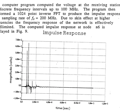
Test Network for Computer Simulation

The computer program computed the voltage at the receiving station at discrete frequency intervals up to 100 MHz. The program then performed a 1024 point inverse FFT to produce the impulse response at a sampling rate of

Is

= 200 MHz. Due to skin effect at higher

frequencies the frequency response of the network is effectively baridlimited. The computed impulse response at node n6 is displayed in Fig. 9.

Impulse Response

1.2~5

1.00t-5

6~6

l00e-6

...:

["

(

·:·..···..···..r·..·

···~

... ···· f·..···..

····!·..···:·

·f..··..····..

···i···

··..

t..···..···

·~

···r..

···~···

....·..·

·!"····..···..

····1···1···

····1

···1"···-;--···:···.:.···1···t···..···:

···r···1···j··· ····!···~···i

.... ···..···t···..···..

I ·· ··..

·7

!

···f···:

···~

..···T..· ···..

····i··..·..····..·..

I···...

··j···....

····1

7-OOe-l 6.DOe-2 ~2 ,... In _4~2 ~ 0 > _l00e-2 '-" Q) ." :J _~2

--

c 0> 1..00e-2 C E Q.D -1~2 -~2 0.0 time (sec)

(18)

Notice the pure delay corresponding to traveling a distance of 180 m from the sending station to the receiving station. Also, immediately following the main impulse, a large second impulse appears with a delay corresponding to traveling a distance of 40 m. This second impulse is due to reflections from the two open circuit transmission lines of 20 m length each ( RG 58/U) which constructively add and propagate to the receiving station.

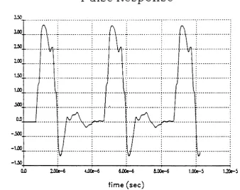
The response of the test network to a series of three pulses, shown in Figure 10, is given in Figure 11. The pulse widths are 1

us .

The rise and fall times are 100 ns and the period is 4 Jls .

Unwindowed Pulse

...: ; : . · . . ·_· ._. ._. · . . · . ... - ~ . · . · . · . · . ... . ~ ; . · . · . · .

...

~ ~

j

~

.

· . :'

...··..1· ···

··t..···..···..·

f'

.

... ···..·t·..·· ·..·

····..t..·· ····..·

·..·t·· ···..··

... ···1··· ···t··· ; .

5.DO ....-- •.••••••..•••••••••••••••~_••••••••.••••••••••.•••••~_••••••••.••••••••••••••••

· . . . .

• I • • •

4..50 _{... -:-}: _:: .:_-:- _:: _{···7···}:

· . . . . · . . . . ·- . . ... . · . _.... . ~ ; .:. . · . . · . . · . . · . . · . . •.00 ,-... ~ rn ~ 0 ₁₀₀ > '-" a> _2!D -c ::s

-

_c 2.00

0»

C

1~

E

1.00 ....•... . •••...~...•.. . .•..•.~...•.••..••.•...••...~_.. _ .

· . :

!JtJ

1 L

~

.

0.0

~

j

Q.D lOOe-6 .-OO!-6 6lX)e-6 8.~6 tOOt-5 1.2Ot-5

time (sec)

(19)

Pulse Response

150 1~5 l.oc.-5 ...

,

_· :_. ;_. :_. . · . . . · . . . · . . . · . . . ... ! . . . • . . .: ! : . · . . . ·_· ._. ._. ._. · . . . · . . ...: : . · . . . · . . . · . . . · . . . · . . . ..._· . -..

_

. . . . · . . . · . . . · . . . · . . . · . . . ..._· .

_

. . . . · . . . · . . . · . . . . . . ...: ; . · . · . · . ·_· ._. ...._ -: - ~ : ~ _..-: . · . . . . : : : : : · . . . . · . . . . ...: :- : : . · . . . · . . . · . . . · . 0.0 lOO

.5CX) •••••••••••••••••••••••••••• : •••••••••••••••••••••••••••••• : •••• '" •••••••••

· . ·_· ._. · . · . 1~ 1.00 lOO

-L50-t--_ _---t-_ _~-_-~_--+--

__...- -...

0.0 -.500 -1.00 c en e E

=

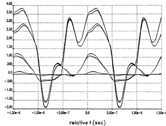
o > '-" CI) -c ::s time (sec)

Figure 12. Pulse response of the test network. The eye diagram corresponding to exciting the network with a pseudo random sequence of pulses with 1 JlS pulse widths, 100 ns rise and fall times and pulse separation of 1.5 JlS is shown in

(20)

Eye Diagranl

I

8..00e-7

...

I

SJX)e-7

2JX)e-7

0.0

-2.OOt:-7

...': : .

· .

i i

~7 -t00e-7

.··..r..··..···..

r···..··..

·r..·....·..·:···....··..

·~

..····..

···i..··.... .;... ..:

l50 .

100

2.50

~ l.OO

rn

~

0 1.50

>

'-'"

CD _,.00

-0

::5

~

s»

-

0-E _0.0

C

-:nJ

relativet (sec)

Figure 12. Eye diagram of the test network

An interesting phenomenon associated with complex transmission line systems is that while reliable communication to one node is possible, another node may exhibit significantly lower

(21)

Eye Diagram

1~-6 1.00e-6 5.00e-7 0.0 -~.00e-7 · . ..._· _. _. _. _.. · . . . . · . . . . · . . . . ..._· _. _. . · . . · . . · .. .. ... -tJX)e-6 1.00 4.00 . 1~ .500 l30 100 2.50 loo

-lOO...- +-- +---_ _- . . --+ --+ ---t

-1.50e-6

-1.50

-1.00 .:_· ;_. _.: :_. :._. :_.

· . . . . .

• til •• •

... ! •...•o• • • : • • • • • • • • • • • • • • • •! : !

· . . . . . . . . . . . . . . . . -.500 c. E o

relativet(sec)

Figure 13. Eye diagram at node n2

1.5Oe-6 1.GOe-6 ~00e-7 0.0 · . ....:._· : . . · . · . · . · . -5.DOe-7 -1.00e-6

J...5£) •••••••••••••••; : ••••••••••

:: 0·.0:::::::::::

i::::::::::::::

t:::·:..

0. 00::

t: .

0:::::::::::;::::::::::

:::::r::

o

-1..004- + - - - - i - - - t - - - t - - - t - - - 1

-t.5Oe-6 -.500

:: :::::::::::::::I:::::

:::::::::r:::::::::::

o

• •

~::::::::::

: : : : : : \ : : : : : : : : : : : : : : :

r:::::::::::···

1

· . · . · . 1.50 ~ rn

=

o >

' - "

CD ""0 :J

....

0.. E o

relativet(sec)

(22)

Eye

Diagram

1~ 1.00e-6

5.00e-7

... i : -0• •;

. ._. ._.

0.0

···..···r· ·

~ ~

.

-S1JOe-7

-1.00e-6 150

aso

1OO ••• •..···r···..·..

·f···..·..··· :

.

-1.50-t--_ _- - t --t- -+-_ _--+ -+-_ _---i

-1.5Oe-6

-1.00

+

\...

.

;

:

· . · . · . · . ~ 2.00 In

==

0 1.50

> "-" Q) _1.00 -0 ~

....

_.500 a. E _0.0 c -.500

relativet(sec)

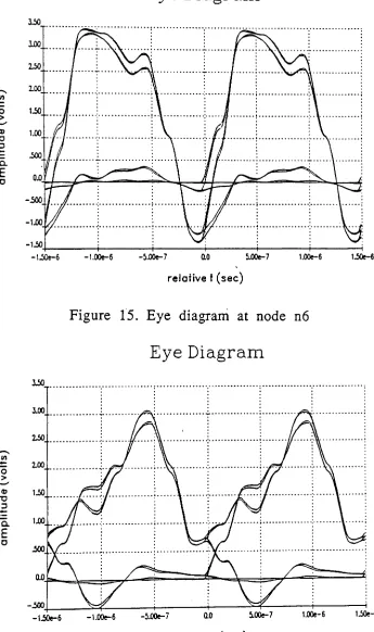
Figure 1"5. Eye diagram at node n6

Eye

Diagram

aso . . . = : .

. ,_. ._. . . 1.5Oe-6 1.00e-6 5.00e-7 0.0 ; .,:._. :_. . -S.00e-7 -1.00e-6 3.00 •..•....•..•... _ .

-!ltJ,-I--_ _~~---+---t---~"f---t---1

-1.50e-6 ,... In ~ _2.00 0 > ""-"" Q) _1.50 -0 :J

...

a. 1.00 E 0

relative t(sec)

(23)

The results presented above were obtained from the program CAPNET written by Joseph Hall [5] which solves complex

transmission line networks based on the technique presented in this paper. Using CAPNET a complicated network is graphically captured using flexible graphical editing capabilities. The program also models junctions such as bends, "tees", and transitions between different

types of transmission lines. The plots presented in this paper are from sessions in CAPNET in which the user can change parameters, plot the results, and obtain hard copies of the plots without leaving the program. CAPNET uses GKS for its interactive graphics and workstation independent capabilities.

Finally in Fig. 17, the voltage distribution along the 50 m cable connecting the receiving station to the main RG 8/U coaxial cable transmission line is shown at a frequency of 10 MHz. Note the standing wave pattern and loss associated with skin effect in the cable. The source was 5 volts. ~

Voltage Distribution

1.60

.&lO

o.o~_-r--_~_"""'-_~_~_"""-_-t--_"""""'_-+---4

0.0 5.00 10.0 15.0 20.0 25.0 30.0 35.0 40.0 ~5.D ~.o

2.00 • • • • • • • • • :• • • • • • • • • •-• • • • • • • • • •-• • • • • -• • - , - • • • • • • • • - , - • • • • • • • • eo· - • • • • • • • • • • - • • • • • • • • • •~• • • • • • • • • :

· . . . .

· . . . '" . . . . .

· . _{. .}. . . ._.

.-iOO

1.00

.600

1.80

c

C'>

o

E

x (meters)

(24)

VIII. Conclusions

In this technical report, a computer program is described which simultaneously solves for all nodes within complex networks of

transmission lines. A tree data structure was introduced for

representing the network in the computer. Recursive procedures

were presented for traversing the tree data structure to compute the impedance, voltage and current at each node within the network. Simulation results were then presented in which the impulse

response of a test 'network composed of transmission lines of various

characteristics and lengths was computed. The impulse response was

then related to the network in terms of the predicted reflections and delays.

The program efficiently solves complex transmission line networks

and has applications in the area of Computer Aided Design (CAD) of

digital communication networks. Specific applications include the

Distribution Line Carrier Network, the digital subscriber loop, and Local Area Networks.

IX. References.

[1] D.G. Messerschmitt, "Transmission line modeling program written

in C,"IEEE Journal on Selected Areas in Communications,Vol. SAC-2,

pp. 148-153, January 1984.

[2] .Dworsky, Lawrence N, Modern Transmission Line Theory and