Enhancement of Optimization Problem in Radio
Networks using Genetic Algorithm
Monika Srivastava
S.P.Tripathi
G.B.T.U., Lucknow G.B.T.U., Lucknow
A.K.G.E.C., Ghaziabad I.E.T., Lucknow
ABSTRACT
The availability of mobile information systems is being driven by the increasing demand to have information available for users at any time. As the availability of wireless devices increases, so will the load on available radio frequency resources. The radio frequency spectrum is limited, thus there will be a need to effectively manage these resources.
This paper studies the application of the genetic algorithm in optimizing cellular radio networks. The aim of the algorithm is to allocate the available frequency channels in such a way that the average quality of the signals that the mobile stations receive is maximized, while meeting the minimum requirement even for the worst signals.
In this study, a genetic algorithm for solving the channel allocation problem is implemented in MATLAB environment and the parameters of the genetic algorithm are tuned so that the algorithm converges nicely.
General Terms
Mobile Computing, Wireless Network
Keywords
Genetic Algorithm, Channel Allocation.
1.
INTRODUCTION
A cellular network is a mobile network in which radio resources are managed in cells. A cell is a two-dimensional area bounded logically by an interference threshold. By exploiting the ability minimize the co-channel interference, one can ensure that mobile stations will receive a strong signal to communicate. Further, channels can be assigned in a way that maximizes their availability at a future time. A number of decisions have to be made in the process of frequency assignment. Thus, a choice must be made intelligently that minimizes interruption to services [1, 2, 3]. The received signal quality in cellular radio networks depends basically on three things: the received signal power, the interference power, and the level of background noise.
1. The received signal power depends on the distance between the transmitter and the receiver and this can not be optimized because mobile can be anywhere in the region.
2. The level of background noise is something that cannot be changed. Because we do not have control on other traffic.
3. Therefore, optimizing the signal quality must be done by minimizing the interference. So co-channel interference is taken into account.
The sources of the interference that the mobile stations receive are the other connections on the same frequency channel in the other parts of the network. The closer the interferer, the higher the interference it causes. This gives
rise to a question of how the available frequency channels should be allocated to the mobile stations so that the performance of the network is optimized. In any matured cellular network the number of users is much larger than the number of frequency channels. Therefore, each channel is shared by several users, but if their connections do not take place too close to each other, then they do not interfere each other too much.
2.
CHANNEL ALLOCATION
Channel allocation deals with the allocation of channels to cells in a cellular network. Once the channels are allocated, cells may then allow users within the cell to communicate via the available channels. Channels in a wireless communication system typically consist of time slots, frequency bands and/or CDMA pseudo noise sequences, but in an abstract sense, they can represent any generic transmission resource.
2.1
The Channel Allocation Problem
With the significant increase in the number of the mobile users, the number of mobile devices (hosts) has increased. Due to this increasing load, the number of mobile hosts that could not connect to the destination (called blocked hosts) has also increased. There are two ways to solve this problem. The first is by increasing the number of channels, but that incurs certain costs. The other way is to utilize the current infrastructure efficiently and try to maximize the uses of the available infrastructure so that the best performance can be achieved. The latter is obviously preferable, as it is always cost effective to utilize the available resources effectively than to add more bandwidth. The channel allocation problem addresses the effective channel utilization in a cellular network.2.2
Channel Allocation Schemes
interference occurs. The minimum distance necessary to reduce co-channel interference is called the reuse distance. The reuse distance is defined as the ratio of the distance, D, between cells that can use the same channel without causing interference and the cell radius, R. Note that R is the distance from the center of a cell to the outermost point of the cell in cases when the cells are not circular.
Fig 2: Cell Architecture
Adding bandwidth to a mobile network is an expensive operation. When developing a mobile network‟s infrastructure, wasting bandwidth should be avoided because it is very costly. Thus, the objective is to try and get the most out of the minimum infrastructure. The same problem applies to a mobile network that is already installed, where it is cheaper to utilize the available resources more effectively than to add more bandwidth.
The channel allocation problem involves how to allocate borrowable channels in such a way as to maximize the long term and/or short-term performance of the network. The performance metrics that can be used to evaluate the solutions proposed will be primarily the number of hosts blocked and the number of borrowings. A host is blocked when it enters a cell and cannot be allocated a channel. Obviously, the more hosts that are blocked, the worse will be the performance of the network. The other major metric is the number of channel-borrowings. This should be minimized because channel borrow requests generate network traffic. There are other metrics that can be used to evaluate the performance of the solution such as the number of “hot cells” that appear in a cellular environment. There are three major categories for assigning these channels to cells (or base-stations). They are
Fixed Channel Allocation,
Dynamic Channel Allocation and
Hybrid Channel Allocation which is a combination of the first two methods.
2.2.1
Fixed Channel Allocation
Fixed Channel Allocation (FCA) systems allocate specific channels to specific cells. This allocation is static and can
not be changed. For efficient operation, FCA systems typically allocate channels in a manner that maximizes frequency reuse. Thus, in a FCA system, the distance between cells using the same channel is the minimum reuse distance for that system. The problem with FCA systems is quite simple and occurs whenever the offered traffic to a network of base stations is not uniform. Consider a case in which two adjacent cells are allocated N channels each. There clearly can be situations in which one cell has a need for N+k channels while the adjacent cell only requires N-m channels (for positive integer‟s k and m). In such a case, k users in the first cell would be blocked from making calls while m channels in the second cell would go unused. Clearly in this situation of non-uniform spatial offered traffic, the available channels are not being used efficiently. FCA has been implemented on a widespread level to date.
2.2.2
Dynamic Channel Allocation
Dynamic Channel Allocation (DCA) attempts to alleviate the problem mentioned for FCA systems when offered traffic is non-uniform. In DCA systems, no set relationship exists between channels and cells. All channels are kept in a central pool and are assigned dynamically to radio cells as new calls arrive in the system. After a call is completed, its channel is returned to the central pool. In DCA, a channel is eligible for use in any cell provided that signal interference constraints are satisfied. Because, in general, more than one channel might be available in the central pool to be assigned to a cell that requires a channel, some strategy must be applied to select the assigned channel. There are two problems that typically occur with DCA based systems.
First, DCA methods typically have a degree of randomness associated with them and this leads to the fact that frequency reuse is often not maximized unlike the case for FCA systems in which cells using the same channel are separated by the minimum reuse distance.
Secondly, DCA methods often involve complex algorithms for deciding which available channel is most efficient. These algorithms can be very computationally intensive and may require large computing resources in order to be real-time.
2.2.3
Hybrid Channel Allocation
The third category of channel allocation methods includes all systems that are hybrids of fixed and dynamic channel allocation systems. Several methods have been presented that fall within this category and in addition, a great deal of comparison has been made with corresponding simulations and analyses. We will present several of the more developed hybrid methods below.
the borrowed channel because of co-channel interference. This can lead to increased call blocking over time. To reduce this call blocking penalty, algorithms are necessary to ensure that the channels are borrowed from the most available neighboring cells; i.e., the neighboring cells with the most unassigned channels.
Two extensions of the channel borrowing approach are Borrowing with Channel Ordering (BCO) and Borrowing with Directional Channel Locking (BDCL).
Borrowing with Channel Locking was designed as an improvement over the simpler Channel Borrowing approach as described above. BCO systems have two distinctive characteristics:
i. The ratio of fixed to dynamic channels varies with traffic load.
ii. Nominal channels are ordered such that the first nominal channel of a cell has the highest priority of being applied to a call within the cell.
The last nominal channel is most likely to be borrowed by neighboring channels. Once a channel is borrowed, that channel is locked in the co-channel cells within the reuse distance of the cell in question. To be "locked" means that a channel can not be used or borrowed. Zhang and Yum [6] presented the BDCL scheme as an improvement over the BCO method. From a frequency reuse standpoint, in a BCO system, a channel may be borrowed only if it is free in the neighboring co-channel cells. This criterion is often too strict.
In the BCO strategy, a channel is suitable for borrowing only if it is simultaneously free in three nearby co-channel cells. This requirement is too stringent and decreases the number of channels available for borrowing. In the Borrowing with Directional Channel Locking (BDCL) strategy, the channel locking in the co-channel cells is restricted to those directions affected by the borrowing. Thus, the number of channels available for borrowing is greater than that in the BCO strategy. To determine in which case a “locked” channel can be borrowed, “lock directions” are specified for each locked channel. The scheme also incorporates reallocation of calls from borrowed to nominal channels and between borrowed channels in order to minimize the channel borrowing of future cells, especially the multiple-channel borrowing observed during heavy traffic. A disadvantage of BDCL is hat the statement "borrowed channels are only locked in nearby cells that are affected by the borrowing" requires a clear understanding of the term "affected." This may require microscopic analysis of the area in which the cellular system will be located. Ideally, a system can be general enough that detailed analysis of specific propagation measurements is not necessary for implementation.
3.
GENETIC ALGORITHM
A genetic algorithm (GA) is a procedure used to find approximate solutions to search problems through application of the principles of evolutionary biology. Genetic algorithms use biologically inspired techniques such as genetic inheritance, natural selection, mutation, and sexual reproduction (recombination, or crossover). Along with genetic programming (GP), they are one of the main classes of genetic and evolutionary computation (GEC) methodol
ogies.
YES
NO
Fig 3: Flow Chart of a General form of Genetic Algorithm
Genetic algorithms are typically implemented using computer simulations in which an optimization problem is specified. For this problem, members of a space of candidate solutions, called individuals, are represented using abstract representations called chromosomes. The GA consists of an iterative process that evolves a working set of individuals called a population toward an objective function, or fitness function. Traditionally, solutions are represented using fixed length strings, especially binary strings, but alternative encodings have been developed.
The evolutionary process of a GA is a highly simplified and stylized simulation of the biological version. It starts from a population of individuals randomly generated according to some probability distribution, usually uniform and updates this population insteps called generations. Each generation, multiple individuals are randomly selected from the current population based upon some application of fitness, bred using crossover, and modified through mutation to form a new population.
3.1
Initialization
In the initialization, one generates, often randomly, a population from which new generations are formed. At this point one also needs to de-₃ne the terminating condition so that the algorithm stops running once an acceptable solution is found.
3.2
Crossover
Crossover is one of the genetic operators used in producing new candidates using the features of the existing ones. The crossover procedure is illustrated in Figure below.
1 1 1 1 1 1 1 1 1
Initialization
Carry the Crossover Procedure with a defined Probability
Mutate with a defined Probability
Is the termination condition met ?
Terminate Select the strongest
Pick up Two Parents
Select the Crossover Points
Switch the values
Fig3.2: Crossover Procedure
The crossover procedure consists of three parts. First one selects two parents from the population. Then the crossover points are selected. The selection of crossover points is done at random, usually so that the distribution from which the points are drawn from is uniform. In figure 3.2 two crossover points are marked with lines. Once the points are de₃ned two offsprings are generated by interchanging the values between the two parents as illustrated in the figure 3.2.In the genetic algorithm crossover is the operator that spreads the advantageous characteristics of the members around the population.
3.3
Mutation
In the genetic algorithm mutation is the operator that causes totally new characteristics to appear in the members of the population. In many cases the mutations, of course, result in offsprings that are worse than the other members, but sometimes the result has such characteristics that make it better. Figure below demonstrates the mutation operation.
Fig 3.3: Mutation Procedure
First, one selects a member from the population to be mutated and a point of mutation. Then the values at the point of mutation are replaced by another value that is picked randomly from the set of all possible values.
3.4
Evaluation
After the population is manipulated using the genetic operators, the fitness of each of the new offspring‟s is evaluated. For this one needs to have a numerical function, fitness function.
3.5
Selection
In the selection the weakest individuals in the population are eliminated. The fit offspring‟s survive to the next generation.
This chapter begins with a survey of GA variants: the simple genetic algorithm, evolutionary algorithms, and extensions
to variable-length individuals. It then discusses GA applications to data mining problems, such as supervised inductive learning, clustering, and feature selection and extraction. It concludes with a discussion of current issues in GA systems, particularly alternative search techniques and the role of building block (schema) theory.
4.
TYPES OF GA
The simplest genetic algorithm represents each chromosome as a bit string (containing binary digits: 0s and 1s) of fixed-length. Numerical parameters can be represented by integers, though it is possible to use floating-point representations for reals. The simple GA performs crossover and mutation at the bit level for all of these.
Other variants treat the chromosome as a parameter list, containing indices into an instruction table or an arbitrary data structure with pre-defined semantics, e.g., nodes in a linked list, hashes, or objects. Crossover and mutation are required to preserve semantics by respecting object boundaries, and formal invariants for each generation can specified according to these semantics. For most data types, operators can be specialized, with differing levels of effectiveness that are generally domain-dependent.
5.
APPLICATIONS
Genetic algorithms have been applied to many classification and performance tuning applications in the domain of knowledge discovery in databases (KDD). De Jong et al. produced GABIL (Genetic Algorithm-Based Inductive Learning), one of the first general-purpose GAs for learning disjunctive normal form concepts.[7] GABIL was shown to produce rules achieving validation set accuracy comparable to that of decision trees induced using ID3 and C4.5. Since GABIL, there has been work on inducing rules and decision trees using evolutionary algorithms. Other representations that can be evolved using a genetic algorithm include predictors and anomaly detectors. Unsupervised learning methodologies such as data clustering also admit GA-based representation, with application to such current data mining problems as gene expression profiling in the domain of computational biology. KDD from text corpora is another area where evolutionary algorithms have been applied.
GAs can be used to perform meta-learning or higher-order learning, by extracting features, selecting features, or selecting training instances. They have also been applied to combine, or fuse, classification functions.
6.
FUTURE TRENDS
Some limitations of GAs are that in certain situations, they are overkill compared to more straightforward optimization methods such as hill-climbing, feed forward artificial neural networks using back propagation, and even simulated annealing and deterministic global search. In global optimization scenarios, GAs often manifests their strengths: efficient, parallelizable search; the ability to evolve solutions with multiple objective criteria and a characterizable and controllable process of innovation.
Several current controversies arise from open research problems in GEC:
• Selection is acknowledged to be a fundamentally important genetic operator. Opinion is, however, divided over the importance of crossover verses mutation. Some argue that crossover is the most important, while mutation is only necessary to ensure that potential solutions are not lost.
2 2 2 2 2 2 2 2 2
1 1 1 1 1 1 1 1 1
2 2 2 2 2 2 2 2 2
1 1 2 2 2 1 1 1 1
2 2 1 1 1 2 2 2 2
1 1 1 1 1 1 1 1 1
Others argue that crossover in a largely uniform population only serves to propagate innovations originally found by mutation, and in a non-uniform population crossover is nearly always equivalent to a very large mutation (which is likely to be catastrophic).
• In the field of GEC, basic building blocks for solutions to engineering problems have primarily been characterized using schema theory, which has been critiqued as being insufficiently exact to characterize the expected convergence behavior of a GA. Proponents of schema theory have shown that it provides useful normative guidelines for design of GAs and automated control of high-level GA properties (e.g., population size, crossover parameters, and selection pressure). Recent and current research in GEC relates certain evolutionary algorithms to ant colony optimization.
7.
THE NETWORK
7.1
Topology of Network
The network consists of 19 base transceiver stations, each serving one cell with a radius of one kilometer. The cells form a hexagonal grid. In each cell there are three mobile stations. The locations of the mobiles are chosen at random from a distribution that is uniform over the corresponding hexagonal cell.
Fig 7.1: Topology of Network
7.2
Propagation Modeling
The amount of attenuation that the signal experiences in the air interface between the transmitter and the receiver, path loss, can be calculated using the following model[4]:
Lp = 40(1 – 0.004∆h) log(R) -18 log (∆ h) + 21 log (f) + 80Db
Where,
Lp is the attenuation in dB,
h is the height of the base station antennas above the rooftop level in meters,
R is the distance between the transmitter and the receiver in kilometers,
f is the carrier frequency in MHz
This formula gives the attenuation on average, i.e., possible fading effects are not taken into account.
Assuming h equal to 15 meters and a UMTS carrier frequency of 2000 MHz and adding the antenna gain of 9 dB, we get the total loss, L, as a function of R only:
L = 119.1 + 37.6 log (R)
Furthermore, the signal power at the receiver, PR , is
PR = PT , L
Where PT is the transmission power of 43 dBm.
The quality of the received signal not only depends on the received signal power, PR, but also on the amount of interference and noise. For this, a concept of signal-to-interference-and-noise ratio, SINR[5] is needed:
SINRk = PR,C [mW]/ ∑iЄI PR,I [mW] + N0 [mW]
Where,
SINRk is the SINR for mobile station k on the linear scale, PR,C [mW] is the received carrier power in mW,
PR,C [mW] is the received power of the interfering signal arriving from base station i in mW,
I is the group of connections using the same frequency channel,
N0[mW] is the thermal noise in mW.
Switching between the linear (mW) and decibel (dB/dBm) scales can be done with the following, well known relations:
x[dBm] =10 X log (x[mW]) x[mW] =10^(x[dBm]/10)
8.
IMPLEMENTATION
8.1
Initialization
The population is formed so that there are 12 individuals that are represented as vectors. The length of each of the individuals is the same as the number of mobile stations connected to the network. The ith value in the vector gives the frequency channel that mobile station i is using.
Because one of the purposes of this project is to study the performance of the genetic algorithm, the individuals are initialized corresponding to a worst case situation, i.e., such case in which all the mobile stations are allocated to the same channel. In this case the one selected is the channel number one. The terminating condition is defined by the number of generations to be produced. In order to better compare the different evolutions the length of the run should be constant. Later, this „age‟ of the population is selected so that the algorithm works optimally.
8.2
Crossover
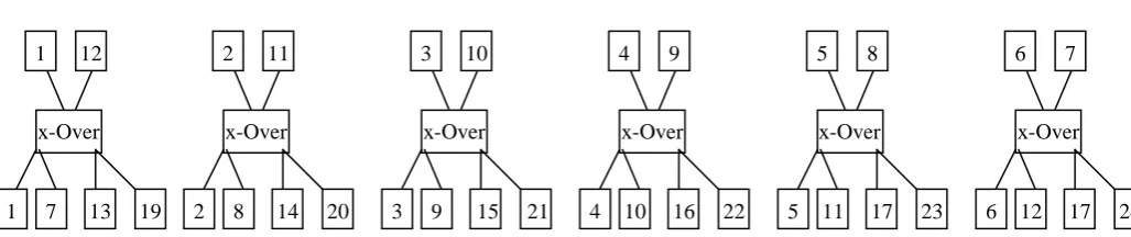
Fig 8.2: Crossovers
Overall, the size of the population of children is 24. The order of the children is mixed so that the siblings are not always next to each other in the new generation, see Figure 8.2.
In crossover there is also a probability, namely crossover probability, involved. With this probability the crossover is done, otherwise the children are identical to their parents.
8.3 Mutation
Mutation is carried out for the individuals after the crossover procedure. In mutation one changes one of the values in a vector representing an individual. This is carried out with a pre-defined probability, mutation probability. Just like crossover probability, this mutation probability is one of the parameters of the algorithm.
8.4 Evaluation
A smart channel allocation has basically two characteristics. Firstly, the average signal-to-interference-and-noise ratio, SINR that mobile stations receive must be as high as possible.
This reflects the overall performance of the network. On the other hand, the minimum SINR requirement for all the users must be met. In this case the minimum requirement is set at SINR = 9 dB.
The fitness function in this case has the following form:
Fitness = SINR + penalty + jitter Where
SINR is the SINR that the mobile stations experience on average in dB.
Penalty decreases the fitness is some mobiles experience a SINR that is lower than 9 dBm
Jitter adds randomness.
The Penalty and Jitter, respectively, are calculated with the following formulas: Penalty = -5 x (9 – min ( 9, min (SINR))
Jitter = (10 / #G+1) * U Where
#G is the order number of the corresponding generation, and
U is a random number from a uniform distribution between 0 and 1.
Obviously, the effect of jitter becomes negligible in higher generations.
In the beginning however, when #G is small, jitter has an effect on the fitness: this way none of the individuals do not start to dominate the others too much at a point when all of the individuals are equally bad.
8.5 Selection
A simple selection scheme is utilized of the 24 individuals the worse half is eliminated and the rest will contribute to the next generation.
8.6 GA Parameter Tuning
There are three parameters related to the implementation of the genetic algorithm that must be tuned before the algorithm is used. These parameters are crossover probability, mutation probability and the number of generations to be produced. Crossover and mutation probability affect on how the population evolves in time, and the number of generation must be chosen so that the optimal, or at least a good one, solution is found.
8.6.1 Crossover Probability
In order to study the effect of crossover probability on the evolution, the algorithm is run with different crossover probabilities ranging from 0.2 to 1.0. For these runs the mutation probability is equal to 0.4, and the maximum fitness for each generation is traced. The results are shown in Graph below.
From Graph 8.6.1 it can be seen that with all the values of crossover probability the evolution converges pretty nicely. Even though there are some differences between the runs, the time of convergence seems to be mostly a matter of luck. With the crossover probabilities closer to one the evolution converges slightly faster, and therefore, a value of 0.8 is chosen to be the crossover probability with which the final results are generated.
Fig 8.6.1: Evolution of fitness with different crossover probabilities ranging from 0.2 to 1.0
A probability of 1.0 is not selected because it seems to
x-Over 1 12
1 7 13 19
x-Over 2 11
2 8 14 20
x-Over 3 10
3 9 15 21
x-Over 4 9
4 10 16 22
x-Over 5 8
5 11 17 23
x-Over 6 7
behave somewhat chaotically even though it converges fastest.
8.6.2 Mutation Probability
The effect of mutation probability is studied similarly to that for crossover probability in the previous subsection. The algorithm is run with five different mutation probabilities from ranging 0.2 to 1.0. The maximum fitness as a function of generation is presented in Graph below for all of the five runs.
Graph 8.6.2 shows that the evolution of the population significantly depends on the mutation probability. With high mutation rate the better values of fitness are reached faster but, on the other hand, the population acts chaotically and the maximum is not reached in the later generations. This shows that if the mutation probability is very high, then some of the advantageous characteristics of the generations are eliminated by mutation and the fitness of the population does not
Fig 8.6.2: Evolution of fitness with different mutation probabilities ranging from 0.2 to 1.0
Converge. With lower values of mutation probability the fitness evolves more slowly but the populations do not act chaotically. Therefore, the requirement of convergence is met.
A good compromise between fast evolution and nice convergence seems to be at a mutation probability of 0.4.
8.6.3 Number of Generations
The number of generation to be produced is selected so that the algorithm almost always converges to a good value of fitness. From Graph 5.2 and Graph 5.3 it can be seen that with reasonable values of crossover and mutation probability the algorithm has easily converged before the 300th generation. To be absolutely sure about the convergence the algorithm is run over 400 generations. Such high confidence margin can be selected because the computations for a system of this size do not take very long for a standard computer of today. For larger systems a less conservative approach may be selected.
9.
RESULTS
The performance of the algorithm in optimizing cellular radio networks is studied in this section. In the system to be optimized there are 19 base stations as illustrated in Graph 7.1 and three mobile stations in each cell. The locations of the mobile stations are chosen randomly, but the coordinates have been the same in every case. Because the mobile positions affect on the fitness, having the locations
unchanged decreases the unwanted variability in the results.
9.1 Maximum Fitness with Different
Numbers of Frequency Channels
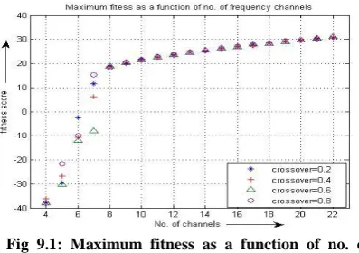
The network is optimized for different number of frequency channels ranging from 5 to 21. Obviously, the larger the number of frequency channels the better should the network perform. The number of interferers is smaller if there are more channels to allocate on.
The results are plotted in Graph 9.1. With the lowest numbers of frequency channels the maximum fitness is very bad. In these cases not all of the mobile stations experience a SINR higher than 9 dB.
Fig 9.1: Maximum fitness as a function of no. of frequency channel
This results in penalty term dominating the fitness. In other words, the mobile stations are packed so tightly on the available frequency channels that it is not possible to meet the minimum requirements for all of them. In cases where there are more than 9 frequency channels the maximum fitness increases with a slope smaller than that with cases where there are less than 9 frequency channels. In this case the minimum requirements of SINR = 9 dB is met for all the mobile stations and the fitness is dominated by the average SINR. The effect of jitter is at most equal to 0.025. Therefore, its effect can not be seen in Graph 9.1.
9.2 Comments on the Performance
One can also see that the resulting maximum fitness increases pretty consistently with the number of frequency channels. This suggests that the algorithm in each run finds a solution that is close to the global maximum. Getting stuck with local maximums would cause inconsistency in the curve.
The number of possible allocations is NM , where N is the total number of available frequencies, and M is the number of mobile stations in the network. In the cases studied here this goes from 457 = 2x1034 to 2157 = 2x1075. Clearly, finding the optimal allocations by going through all the possibilities is not possible, which justifies the use of more intelligent methods such as genetic algorithms. With the implementation of a genetic algorithm used here the number of allocations to be evaluated is 24x400 = 9600 even though a very conservative safety margin was selected for the number of generations to be produced.
10.
CONCLUSION
on solving it. Firstly, the problem was formulated so that solutions can be searched using a genetic algorithm, and then a genetic algorithm was implemented in MATLAB environment. The effects of three parameters, namely crossover probability, mutation probability, and the number of generations to be produced, were briefly studied by tracing the evolution of the initial population with different parameter values. The most suitable parameter values were then suggested. Finally, the performance of an example network was optimized with the genetic algorithm.The application of genetic algorithms in channel allocation optimization sets two requirements for the network. Firstly, the propagation environment must be known and a suitable model for it must be available. In urban areas the attenuation that the signals experience in the air interface is, of course, very different from that in urban areas.
Secondly, the locations of the mobile stations must be known. In most of the networks this is not the case yet. In the near future, however, the locationing services will be launched, which among other things enables the use of more advanced optimization methods.
The results reported show that the genetic algorithm works relatively consistently in optimizing the network. The resulting performance of the network increases with available resources (frequency channels) as expected. The fact that the results form a smooth curve in Graph 9.1 proves that the algorithm in most cases converges close to the global maximum.
Compared to the exhaustive search the performance of the genetic algorithm in finding solutions to this problem is superb; with an exhaustive search the number of points to be checked would have risen at least 2x1034, depending on the case under study, whereas the genetic algorithm found a good solution by checking 9600 points only. Here, the genetic algorithm started with a worse-case initial population; in real life systems this should not be the case, which makes the convergence even faster. Also, for the number of generations less conservative safety margins may be used if the computational power becomes an issue and if it is good enough just to and a good solution and not necessarily the very best one.
11.
ACKNOWLEDGEMENT
I would like to acknowledge my deep sense of gratitude to my Supervisor Dr. Surya Prakash Tripathi, IET
Lucknow for his valuable help, guidance and encouragement for my thesis work. He gladly accepted all the pains in going through my work again and again, and giving me opportunity to learn essential research skills. This work would not have been possible without his insightful and critical suggestions, his active participation in constructing right models and a very supportive attitude. It gives me immense pleasure to express my deep sense of gratitude to my colleagues Ajay Garg and Suyash Kumar for their guidance and encouragement during the course of project work.
Last but not the least, I extend my heartiest gratefulness to my parents for their blessing, husband Devendra for his support and daughter Jhalak for her understanding.
12.
REFERENCES
[1] K. Feher, Wireless Digital Communications. McGraw- Hill, 1995.
[2] M.A.C. Gill and A.Y. Zomaya, Obstacle Avoidance in Multi-Robot Systems. World Scientific, 1998.
[3] A.Y. Zomaya and M. Wright, “Observation on Using Genetic Algorithms for Channel Allocation in Mobile Computing,” IEEE Trans. Parallel and Distributed Systems, vol 13, no. 9, pp. 948-962, Sept. 2002.
[4] European Telecommunications and Standards Institute, ETSI TR 101 112 version 3.2.0, Universal Mobile Telecommunications System (UMTS) Selection procedures for the choice of radio trans-mission technologies for the UMTS, 1998.
[5] Steven W. Smith, The Scientist and Engineer‟s Guide to Digital Signal Processing, California Technical Publishing, 1998.
[6] Zhang, M. and Yum, TS. P., "Comparisons of Channel-Assignment Strategies in Cellular Mobile Telephone Systems", IEEE Transactions on Vehicular Technology, vol. 34, no. 4, November 1989.