Measuring Spatial Correlation of Soil pH and Fe using
Theoretical Variograms
1
Jaishree Tailor; 2 Kalpesh Lad; 3 Ravi Gulati
1
Shrimad Rajchandra Institute of Management & Computer Application, Uka Tarsadia University Bardoli, Gujarat Surat, India
2
Shrimad Rajchandra Institute of Management & Computer Application, Uka Tarsadia University Bardoli, Gujarat Surat, India
3
Department of Computer Science, Veer Narmad South Gujarat University Surat, Gujarat, India
Abstract -The principles of geostatistics states that, locations of data that are close to each other are similar to their neighbors and as the distance between the locations increases, the difference between corresponding data also increases which is known as spatial variability. Therefore this paper measures the spatial variability of soil pH and Fe tested on soil data sets of three talukas of Surat district. Measures of central tendency have been calculated for the soil samples. Empirical and theoretical variograms are calculated and plotted in R 3.2.2.by passing variogram parameters like nugget, sill and range. Further three commonly used variogram models for kriging namely Spherical, Exponential and Gaussian have been fitted for both pH and Fe. The Spherical model was more suitable for pH and Gaussian for Fe. Finally nugget-sill ratio is also calculated to understand the intensity of spatial correlation. The results indicated moderate spatial dependence for pH and strong for Fe in this region.
Keywords - Variogram, Empirical, Theoretical, Spherical, Exponential, Gaussian, Nugget, Sill, Range.
1. Introduction
he assessment of spatial variability amongst the soils of different regions assists the policy makers especially the farmers to take appropriate decisions pertaining to soil status as well as to retain its fertility. Distribution of soil chemical properties, as well its macro and micro nutrients in a region of interest is also an issue of concern to handle toxicity and alkalinity.
Descriptive statistics have been widely used in [1], [2], [3] to study the concentration and correlation amongst different soil chemical properties like pH, EC and OC and its nutrients. [4] Presented spatial distribution of pH and EC for Golestan province using Inverse Distance Weighing, Radial Basis Function and Kriging. Both Spherical and Exponential models were used to compare the prediction accuracy of kriging. Kriging with Spherical model turned out to be best fitted with RMSE = 4.5063, MBE = - 0.0066 & MAE = 1.9772. In [5] ordinary kriging with Spherical and Exponential variograms was compared to IDW and splines to assess the spatial variability of pH, organic matter, Phosphorous and Potassium for Loakkous district
Of Morocco and concluded that Spherical model outperforms for P and Exponential model for pH, OM and K.
Similarly Ordinary Kriging was used in [6] with all the same three variogram models where Spherical and Expo-nential model resulted into 96% and 90% accuracy respectively as compared to Gaussian model. In [7] authors used simple kriging for pH, EC, OM with these three models for spatial correlation and found exponential for pH, OM and spherical best fitted for EC [20].
Thus from the literature review it can be concluded Spherical and Exponential model have been widely used for assessing spatial dependence of soil minerals followed by Gaussian in some of the cases .
A few literature reveals the soil status of Gujarat especially the southern end of the state that is Surat and its talukas. Therefore this paper highlights the use of kriging variogram models namely Spherical, Exponential and Gaussian that can be used for soil data sets of three talukas of Surat district.
2. Semi-variance and Semi-variogram
Kriging uses semi-variance to measure the spatial dependence which is computed in Eq. (1).
1
22
i jh
z x
z x
(1)
where, γ(h) is the semi-variance between known points xi and xj, separated by the distance h; and z is the at-tribute value. If there exist spatial dependence in the data then there will be smaller semi-variance between the known points which are close to each other while the points which are farther apart are expected to have larger semi-variance. The concept of semi-variogram cloud shows all pairs of known points and thus binning is used which to average semi-variance data by distance and direction. The binning process yields bins or well known as grid cells that sorts the pairs of sample points by distance and direction and so the next step is to calculate average semi-variance which is given by Eq. (2).
1
22
1
i i
n
h
z x
z x
h
n
i
(2) where, γ (h) is the semi-variance between the sample points separated by lag h; n is the number of pairs of sample points sorted by direction in the bin; and z is the attribute value. A variogram plots the average semi-variance against the average distance. [8]
3. Variogram Models
A semi-variogram can be used alone so as to measure spatial autocorrelation in the data or spatial region but when interpolations like kriging or its variants are to be employed the semi-variograms have to be fitted with a mathematical function or model [19]. The fitted semi-variogram is then used for estimation of the semi-variance at any given direction. There are several models for fitting semi-variograms, this paper emphasizes on two models namely Spherical and Exponential to study the spatial correlation of pH and Fe. The fitted model can have mainly three possible components: nugget, range and sill. The nugget is the semi-variance at the distance of 0, representing measurement error.
The range is the distance at which the semi-variance starts to level off which corresponds to the spatially correlated portion of the semi-variogram. Once semi-variance crosses the range it observes relatively constant value and starts levelling of which is known as sill and is composed of nugget and partial sill [8], [9].
3.1 Spherical Variogram
The Spherical model has a linear behavior at smaller separation distances near the origin but flattens out at larger distances, and reaches the sill at a, which means it shows a progressive decrease of spatial dependence until some distance, beyond which spatial dependence levels off. Eq. (3) shows the nature of this model.
3
0 0
2
0 0 0 0
3
1
{
,
2
2
h
C
h
h
for h
a
C
a
a
for h
a
(3)
While fitting this model to a sample semi-variogram the tangent at the origin reaches the sill at about two thirds of the range, where 𝛾(ℎ) is the semi-variogram model, ℎ is the Euclidean distance between two points, a is the range and C0 is the nugget. It is a good choice when nugget variance is important but not too large and when range and sill are availed.
3.3 Exponential Variogram
The exponential model as shown in Eq. (4) exhibits a less gradual pattern than the spherical where spatial dependence decreases exponentially with increasing distance and disappears completely at an infinite distance.
0
2 0
1
hh
C
exp
a
(4)The exponential model argues that though the correlations may become arbitrarily small at large distances but they never vanish.
3.2 Gaussian Variogram
The Gaussian model is similar to Exponential model in which the model reaches the sill in case of asymptotically. It is used when the data exhibits strong continuity at short lag distances which means the spatial correlation is very high between two neighboring points.[11].
2 0 2 2 0
1
hh
C
exp
a
(5)become arbitrarily small at large distances, they never vanish in that case exponential model should be preferred.[8][9][10].categories
4. Methodology
The study area selected for this paper confines to secondary datasets obtained for Bardoli, Umarpada and Mandvi talukas of Surat lying to the southern part of Gujarat with minimum and maximum latitude range of 20.97 and 21.51 and a longitude between 72.77 and 73.79 . A total of 103 villages for March 2013 have been selected as sample and were compared with standard limits of the soils (followed by MMSOIL-Gov. of In-dia-2011) [11], [12]. The comparison showed that the concentration of pH and Fe levels were found to be higher and thus selected for study. Then descriptive statistics for these two soil components is calculated in R Studio of R plat-form with the summary ( ) command as shown below. Further both the column summaries of pH and Fe are bonded with cbind ( ).
>library(sp)
> PH<-summary(bmu$pH) > PH
Min. 1st Qu. Median Mean 3rd Qu. Max. 7.341 7.487 7.557 7.550 7.609 7.753
> FE<-summary(bmu$Fe) > FE
Min. 1st Qu. Median Mean 3rd Qu. Max. 9.422 11.160 13.620 13.860 16.560 21.520
> descriptive<-cbind(PH,FE) > descriptive
PH FE Min. 7.341 9.422 1st Qu. 7.487 11.160 Median 7.557 13.620 Mean 7.550 13.860 3rd Qu. 7.609 16.560 Max. 7.753 21.520
4.1 Experimental and Theoretical Variogram for pH
and Fe
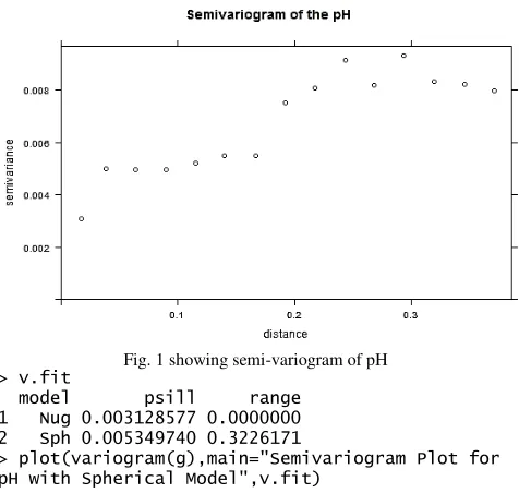
Then the variogram test is carried out on pH and Fe values. Variogram modelling is required to check the spatial correlation (dependence) between the sampling points. First semi-variograms for both pH and Fe were plotted and then fitted with Spherical, Exponential and Gaussian models variograms to understand the spatial correlation in these regions. The variogram which is fitted with a model is known as theoretical variogram. gstat ( ) object is created with pH and Fe as parameter of interest, with locations and whole dataset as arguments. For plot-ting the initial semi-variogram gstat object g is passed to variogram
method which is further passed to the plot method for plotting which is shown in Figure 1 and 4.
The snippet for pH is shown in the code below. This was done using variogram function of gstat package of R under R Studio. After doing so fit.variogram is used to pass the partial sill, model type, range and nugget of semi-variogram and then plotted. Moreover v.fit( ) is used to understand values of each variogram parameters for each model fitted.
> library(gstat)
> g <- gstat(id="pH", formula = (pH)~1, locations = ~Latitude + Longitude, data = bmu)
> plot(variogram(g), main="Semivariogram of the pH")
> v.fit <- fit.variogram(variogram(g),
vgm(0.008,model="Sph",range=0.3,nugget=0.003))
Fig. 1 showing semi-variogram of pH > v.fit
model psill range 1 Nug 0.003128577 0.0000000 2 Sph 0.005349740 0.3226171
> plot(variogram(g),main="Semivariogram Plot for pH with Spherical Model",v.fit)
> v1.fit <- fit.variogram(variogram(g),
vgm(0.008,model="Exp",range=0.3,nugget=0.003)) > v1.fit
model psill range 1 Nug 0.002580614 0.0000000 2 Exp 0.005485665 0.1097757
> plot(variogram(g),main="Semivariogram Plot for pH with Exponential Model",v1.fit)
> v2.fit <- fit.variogram(variogram(g),
vgm(0.008,model="Gau",range=0.3,nugget=0.003)) > v2.fit
model psill range 1 Nug 0.002223708 0.00000000 2 Gau 0.003502571 0.02416968
> plot(variogram(g),main="Semivariogram Plot for pH with Gaussian Model",v2.fit)
> parpH<-rbind(v.fit,v1.fit,v2.fit)
> parpH
model psill range 1 Nug 0.003128577 0.00000000 2 Sph 0.005349740 0.32261711 3 Nug 0.002580614 0.00000000 4 Exp 0.005485665 0.10977571 5 Nug 0.002223708 0.00000000 6 Gau 0.003502571 0.02416968
> parFe<-rbind(v3.fit,v4.fit,v5.fit) > parFe
model psill range 1 Nug 2.761112 0.00000 2 Sph 696.002485 27.25289 3 Nug 2.889416 0.00000 4 Exp 483.328210 12.82728 5 Nug 3.561116 0.000000 6 Gau 11.599149 0.191308
5. Results and Interpretation
Table 1 shows the standard values for nugget sill ratio. The results indicate squared distance with differences calculated for each co-ordinates. Interval of 0.1 with three bins 0.1, 0.2, 0.3 were defined to understand number of pairs within each bin which can be seen in all the figures. The variogram parameters for pH and Fe with the three models appear in the code mentioned above.
Figure 3 plot showing pH with Exponential Model
Fig. 4 plot showing pH with Gaussian Model
Fig. 5 semi-variogram of Fe
Fig. 6 plot showing Fe with Spherical Model
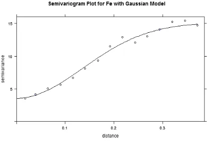
Fig. 8 plot showing Fe with Gaussian Model
Table 1: Standard for Nugget/Sill Ratio
Nugget/Sill Ratio Range
Intensity of Spatial Dependence
<0.25 Strong
0.25-0.75 Moderate
> 0.75 Weak
Table 2: Variogram Parameters for pH with three variogram models
Variogram Parameters
Models
Spherical Exponential Gaussian
C0 0.0031 0.0025 0.0022
C1 0.0053 0.0054 0.00350
C 0.0085 0.0081 0.0057
a 0.3226 0.1097 0.0241
C0/C 0.3690 0.3199 0.3883
SD Moderate Moderate Moderate
Table 3: Variogram Parameters for Fe with three variogram models
Variogram Parameters
Models
Spherical Exponential Gaussian
C0 2.7611 2.8894 3.5611
C1 696.0024 483.3282 11.5991
C 698.7635 486.2176 15.1602
a 27.2528 12.8272 0.1913
C0/C 0.0039 0.0059 0.2348
SD Strong Strong Strong
From the semi-variogram plots it is clear that within a range (distance) of 0.2 which is also known as lag the correlations are positive with a sill value of 0.008 for both Spherical and Exponential model for pH whereas the same sill value with Gaussian is 0.0057 which means correlations are negative and starts diminishing earlier in case of Gaussian than the other two models.
For Fe the two models behave differently with higher sill values of 698 and 486 as compared to 15 of Gaussian. To
check the validity Fe values were log transformed and further variogram modelling was done which also resulted in adverse values for both Spherical (0.45) and Exponential (0.57) model as compared to Gaussian (0.057).
Next is the nugget/sill ratio or spatial dependency (SD) C0 / (C0 + C) which defines the spatial property. The variable is considered as a strong spatial dependence when the value of C0 /(C0 + C) is less than 0.25, a moderate spatial dependence when this value is between 0.25 and 0.75, and a weak spatial dependence when the value is more than 0.75 (Cambardella et al, 1994) [13], [14].
Thus the Spatial dependence of pH is moderate in all the three cases with a ratio of 0.369, 0.319 and 0.388 whereas strong spatial dependence is observed in case of Fe with a ratio of 0.0039, 0.0059 and 0.23 respectively. The summary of the same is presented in Table 2 and 3 for pH and Fe respectively.
Last but not the least observing the curve the spherical model in case of pH is smooth and estimation of individual parameters explicitly is easier from the plot hence spherical model is appropriate as compared to the other two models. Moreover, in case of exponential as well as in Gaussian model the estimation and interpretation of the parameter “range”, r, is more difficult since spatial dependencies never fall to zero thus Spherical model is a choice. But for Fe the scenario is reversed with Gaussian model as a choice over the other two observing from the smoothening of the curve.
6. Conclusion and Future Work
From the nugget sill ratio it can be concluded that Bardoli, Umarpada and Mandvi have moderate spatial dependence for pH values of soil whereas there is a strong spatial correlation between Fe values for these regions. The other important point to be focused is the fitting of variogram models as well as its parameters and curve. The process is rather vague and arbitrary, which can adversely affect the results of kriging and consequently mislead the prediction process of spatial variables [15], [16]. Through this paper the authors have highlighted the problems of vagueness in fitting variogram parameters and model selection process therefore this research can be further extended by proposing alternative solutions towards resolving the above mentioned issues and improve the prediction accuracy [17], [18].
Acknowledgments
References
[1] P. Patel, N. Patel and A. Gharekhan, “Study of basic Soil Properties in Relation with Micronutrients of Mandvi Tahsil near Coastal Region of Kutch Districts”, International Journal of Science and Research, Vol. 3, No. 6 , 2014, pp. 25-28
[2] K. Kalubarme, K. Thakor, N. Dharaiya, V. Singh, A. Patel, K. Mehmood, “ Soil Resources Information System for Improving Productivity Using GeoInformatics Technology” , International Journal of Geosciences, Vol. 5, No. .2014, pp. 771-784
[3] D. Patel, and M. Lakdawala “Study of presence of available phosphorus in soil of Kalol-Godhra taluka territory”, Archives of Applied Science Research, Vol. 5, No. 4, 2013, pp. 24-29.
[4] K. Poshtmasari, Z. Sarvestani, B. Kamkar, S. Shataei and S. Sadeghi, “Comparison of Interpolation Methods for estimating pH and EC in agricultural fields of Golestan province”, International Journal of Agriculture and Crop Sciences, Vol. 4, No. 4 , 2012, pp. 157-167
[5] S. Kamaili, A. Douaik.and L. Moughli, “Soil Fertility Mapping: Comparison of Three Spatial Interpolation Techniques”, International Journal of Engineering Research & Technology, Vol. 3, No. 11 , 2012, pp. 1635-1643 [6] S. Mehdi, S. Ghani, M. Khalid, A. Sheikh and S. Rasheed,
“Spatial Variability Mapping of Soil-EC in Agricultural Field of Punjab”, International Journal of Scientific & Engineering Research, Vol. 4, No. 11, 2013, pp. 325-338 [7] T. Robinson.and G. Metternicht, “Testing the performance
of spatial interpolation techniques for mapping soil properties. Computer and Electronics in Agriculture”, Elsevier, Vol. 50, 2006, pp. 97-108
[8] T. K. Chang, Introduction to Geographical information Systems, Tata Mc Graw Hill, pp. 167-169.
[9] T. Smith (2005). [Online]: Available at http://www.seas.upenn.edu/~ese502/NOTEBOOK/Part_II/4 _Variograms.pdf. [Accessed 23 11 2015].
[10]G. Bohling (2005) [Online] Available: http://people.ku.edu/~gbohling/cpe940/Variograms.pdf. [Accessed 11 9 2015].
[11]J. Tailor and R. Gulati, “Comparing prediction accuracy of OK and RK for the soils of Surat talukas”, Proceedings of Technological Innovation in ICT for Agriculture and Rural Development (TIAR), IEEE, Chennai, 10-12 July 2015,202-207:http://dx.doi.org/10.1109/TIAR.2015.7358558 [12]J. Tailor J, R. Tailor and Gulati R. Application of Ordinary
Kriging on Educational Data using FOSS4G: R Platform, Proceedings of OSGEO-India: FOSS4G 2015- 2nd National Conference “Open Source Geospatial Tools in Climate Change Research and Natural Resources Management”
8-10th June 2015 [Online].
http://papers.foss4gindia.in/2015/11/04/application-of-ordinary-kriging-on-educational-data-using-foss4g/
[13]Baily and Gatrell, [Online].
http://www.math.umt.edu/graham/stat544/varmodel.pdf [Accessed 30 12 2015]
[14]H. Patel, F. Patel, J. Prajapati and J. Tailor, "Regression Kriging : Disguised and Unveiled," Nationa Journal of
System and Information Technology, vol. 6, no. 2, pp. 167-177, December 2013
[15]Caha, Tucek, Vondrakova, Fuzzy Surface Models Based on Kriging Outputs. GIS Ostrava, 2012
[16]Weldon, Lodwick and Santos J., Constructing Consistent Fuzzy Surfaces From Fuzzy Data. CRC Press, 2000 [17]A. Dhar. and R. Patil, “Fuzzy uncertainty Based Design of
Groundwater Quality Monitoring Networks”, Journal of Environmental Research and Development, Vol. 5, No. 3 ,2011, pp. 683-688
[18]R. Sunila, Elaine and Kremenova, “Fuzzy Model and Kriging for imprecise soil polygon boundaries”, Proceedings of 12th International Conference on Geoinformatics, Sweden, June 2004, 489-495.
[19]K. Mulatani, A. Mohammad, M. Jadav and J. Tailor, "Analyzing Spatial Autocorrelation in Distribution of Soil Chemical Properties using Moran'I and Variogram for Talukas of Surat District," National Journal of System and Information Technology, vol. 9, no. 2, pp. 97-107, December 2016.
[20]R. Rathod, G. Kanet, N. Sardhara, H. Solanki, B. Vaghani and J. Tailor , "Application of Ordinary Kriging on Educational Datasets," National Journal of System and Information Technology, vol. 7, no. 2, pp. 91-98, December 2014.
Ms. Jaishree Tailor achieved her M.C.A. degree in 2004 and is pursuing her Ph.D. in Geographical Information Systems from UTU. She is currently working as an Assistant Professor at Shrimad Rajchandra Institute of Management and Computer Application affiliated to Uka Tarsadia University (UTU)-Bardoli Gujarat. She has more than 13 years of experience in management and computer science field. Her area of specialization includes GIS and Open Source Technologies. She has published 7 research papers.
Dr. Kalpesh Lad is working as an Associate Professor at Shrimad Rajchandra Institute of Management and Computer Application affiliated to Uka Tarsadia University (UTU)-Bardoli Gujarat. . He is a Ph.D. and has more than 15 years of experience in academics. His area of interest includes programming languages, system software, digital image processing, and data mining. Till now 2 candidates have completed Ph.D. under his guidance. He has organized and attended many workshops and training programmes. He has 35 plus research papers published to his credit.