1. Comparison of clearance variation using selective assembly and metaheuristic approach

(1)

COMPARISON OF CLEARANCE VARIATION USING

SELECTIVE ASSEMBLY AND METAHEURISTIC

APPROACH

A. Asha1 and J. Rajesh Babu2

I.INTRODUCTION

Producing every component to an exact dimension is impossible because of variation. Variations due to imperfections in the materials, machines, operators, methods, measurements, and so on affect the quality characteristics of products. It is impractical to completely remove such variation even though those components are manufactured by the same process. These variations propagate and accumulate as components are assembled together. An assembly is the process of joining two or more components; the clearance of the assembly depends on the tolerance of the individual components. Generally, mating parts constitute a pair of assembly called female and male parts. The difference between the hole (female) and shaft (male) dimensions of the mating parts is the clearance. The clearance between the mating parts decides the quality of the assembly. The maximum clearance in the assembly is the difference between the maximum dimension of the hole and the minimum dimension of the shaft. The minimum clearance is the difference between the minimum dimension of the hole and the maximum dimension of the shaft.

In practice, minimization of this variation in the assembly clearance, by minimizing the component tolerance by better processes and control measures is found to be very difficult and not cost effective. Nowadays, customer wants quality and trouble free product at a reasonable price. Owing to heavy competition in the market, the

Manufacturers are eagerly looking for a new method to produce a product with high quality and low manufacturing cost. Hence, the manufacturers resort to selective assembly. The use of selective assembly may be a valuable addition to a manufacturing system to improve the quality of a product in a cost effective manner. In selective assembly, the mating parts (i.e., the components) populations are divided into equal number of groups, spanning their dimensional distributions, and selective groups of individual components are chosen and the parts within these groups are assembled at random. This economic method is very useful where the process variation is too high, and

1

Department of Mechanical Engineering Kamaraj College of Engineering and Technology, Virudhunagar, TamilNadu,, India

2

Department of Mechanical Engineering K.L.N. College of Engineering, Pottapalayam, Sivagangai, TamilNadu,, India

DOI: http://dx.doi.org/10.21172/1.83.020

e-ISSN:2278-621X

Abstract- Selective assembly is an approach for reducing the overall variation and thus improving the quality of an assembled product. In this process, components of a mating pair are measured and grouped into several classes (bins) as they are manufactured. The final product is assembled by selecting the components of each pair from appropriate bins to meet the required specifications as closely as possible. This approach is often less costly than a tolerance design using tighter specifications on individual components. It leads to high quality assembly from relatively low precision components. A relatively smaller clearance variation is achieved than in interchangeable assembly, with the components manufactured with wider tolerance.

Selective assembly is carried out in three stages using metaheuristic techniques. These metaheuristic techniques give the best combination. Thus, very high precision assemblies are obtained using the proposed method and minimize the assembly clearance variations and at the same time to minimize surplus parts without sacrificing the benefits of selective assembly. The proposed method is applied for a complex assembly such as ball bearing

(2)

II. OBJECTIVE

In this work, an attempt is made to apply the concept of Selective assembly for a complex radial assembly with three mating parts. Metaheuristic Techniques such as Genetic Algorithm (GA), Simulated Annealing algorithm (SAA) and Memetic algorithm(MA) is proposed to obtain the best combination of selective group to minimize the clearance variation and assembly loss within the specified range.

III. SELECTIVE ASSEMBLY

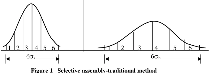
Selective assembly is the method of obtaining high precision assemblies from relatively low precision components. In traditional selective assembly, the dimensional distribution of the mating parts tolerances is divided into a fixed number of groups. The parts are partitioned according to these dimensional groups. The parts in the corresponding groups are assembled interchangeably. The dimensional distribution of the mating parts is considered to be normal and the dispersion is equal to 6. Then 6s is the dimensional distribution of the shaft population and 6h is the

dimensional distribution of the hole population.

For example the hole and shaft population are divided into equal number of parts, (say 6) with their dimensional distributions as shown in Figure 1 . Then the corresponding groups are assembled interchangeably. In this method, there will be no surplus parts, but the clearance variation (cv) will be very high with respect to the difference in

standard deviation of the mating parts.

1 2 3 4 5 6 1 2 3 4 5 6 6s 6h

Figure 1 Selective assembly-traditional method

In the conventional selective assembly method, the components (hole and shaft) are divided into equal number of groups. The components from the corresponding groups are assembled interchangeably, so that closer tolerances could be achieved. For example, a component from hole group 1 and a component from shaft group 2 are taken and assembled. The assembly clearance variation is the difference between the maximum clearance and minimum clearance.

Maximum clearance = selective group number of the hole  group tolerance of the hole

+ selective group number of the shaft  group tolerance of the shaft

Minimum clearance = (selective group number – 1) of the hole  group tolerance of the hole

+ (selective group number –1) of the shaft  group tolerance of the shaft

IV. CASE ANALYSIS

(3)

Figure 2 Ball bearing assembly

The components are manufactured from different processes and the standard deviations of the manufacturing process will be different. The dimensional distribution of the components is equal to the process capability (6σ) of the process. So the process capability (6σ) of the process is considered for analysis. The dimensional distribution or the manufacturing tolerance for inner race, ball and outer race are 12 µm, 6 µm and 24 µm respectively. The dimensional distributions of the components are divided into six equal groups as shown in Figure 3. The group tolerance for component A (Inner race), component B (Ball) and component C (Outer race) are 2 µm, 1 µm and 4 µm respectively

.

Inner Race (A) Ball (B) Outer Race (C)

1 2 3 4 5 6 1 2 3 4 5 6 1 2 3 4 5 6 12 µm 6 µm 24 µm

Figure 3 Dimensional distributions of the components for the ball bearing assembly

When the components are assembled interchangeably the clearance variation of the population is 42 µm i.e. (12+6+24). When assembled using traditional system of selective assembly the maximum clearance and minimum clearance is calculated with the formula mentioned in Section III. The assembly clearance is calculated as shown below for group 1 of ball bearing assembly

Maximum clearance = 1 × 2 + 1 × 1+1 × 4 = 7 µm

Minimum clearance = 0  2 + 0 1 + 0  4 = 0 µm

The assembly clearance is calculated as shown below for group 6 of ball bearing assembly

Maximum clearance = 6 × 2 + 6 × 1 +6 × 4 = 42 µm

7. 5 mm

35 mm

7..5 mm

Outer race (C)

Inner race (A)

(4)

interchangeable system. The precision decreases from first group to the sixth group. The only benefit in the existing method is that the precision assemblies can be segregated. In selective assembly, the corresponding groups are assembled interchangeably. The clearance variation for each assembly group is 7 µm. But for the population it is 42 µm. Instead of assembling corresponding selective groups, the optimum selective group combination is obtained using Metaheuristic Techniques. In selective groups, the number of components in each selective group is not the same. In the proposed method, all the components are assembled in three stages and so there will be no surplus parts. The assembly clearance variation achieved is less than interchangeable systems. A high precision assembly is achieved with the same components using a better combination obtained through this proposed method.

V. SELECTION OF BEST COMBINATION USING GA

GA is used as a tool to find the best combination of the selective group of components for obtaining minimum assembly clearance variation in selective assembly. In the initialization module some possible combination of the selective group numbers are represented as chromosomes. This is the initial population. GA is used to find the best combination of selective groups from this population. The primitive search process of the proposed GA is schematically given in Figure 4.

Input Module

The input data are,

i) Number of components (N)

ii) Number of groups in a component (Group_size) iii) Number of chromosomes in initial population (pop_size)

Example:

Input values for FIRST stage,

i) N = 2

ii) Group_size = 6 (1,2,3,4,5,6) iii) pop_size = 10

Input values for SECOND stage,

i) N = 2

ii) Group_size = 4 (2,3,4,5) iii) pop_size = 10

Input values for THIRD stage,

i) N = 2

ii) Group_size = 2 (3,4) iii) pop_size = 10

The number of times the whole process (iteration) of evaluation, selection, crossover and mutation is to be repeated until the objective criterion gets the best value. The best chromosome in each iteration is stored and best among the best stored is the optimal one. The best chromosome having minimum clearance variation is given as the output. The best chromosomes for all the three stages are given in the following Tables 1 to 3. The output shown in Table 4 is obtained by writing a “C” program for the Genetic algorithm

Table 1 Best combinations for the first stage

Component A Component B Component C

1 4 5 3 2 6 2 5 6 3 1 4 6 4 2 3 5 1

Table 2 Best combinations for the second stage

Component A Component B Component C

4 5 2 3 4 5 2 3 3 2 5 4

Table 3 Best combinations for the third stage

Components A Components B Components B

(5)

No

INPUT MODULE

Number of components, Number of chromosomes, Number of groups in each component.

INITIALIZATION MODULE

Collection of some possible chromosomes.

EVALUATION MODULE

for (chromosome =1 to pop_size)

find the fitness parameter values (Clearance variations) Clearance variations (fit(c)) = Max clearance – Min clearance;

NEW POPULATION GENERATION MODULE Selection ( )

for (chromosome =1 to pop_size)

newfit(c) = e (-k fit(c) ) (k=0.05 constant) c=pop_size

p(c) = newfit(c) /  newfit(c) c=1

c=pop_size

cp(c) =  p(c)

c=1

{

generate random no. ‘r’; select ‘c’ satisfying cp(c-1) < r <= cp(c) and label c’

}

Crossover ( )

for (chromosome=1 to pop_size) {

generate random no. ‘r’; if(r <= p_cross (0.60))

Select c and label c

do

{ get parents c and c + 1; do three point cross over;

} }

Mutation ( )

for (chromosome =1 to pop_size) { for (j=1 to m) generate random no. ‘r’;

if (r <= p_mut (0.05)) Mutate gene ‘g’;

}

Check for Termination

OUTPUT MODULE Print the best combinations and its

clearance variation

(6)

Table 4 Clearance Variation for three stages

S.No. Stages Clearance Variation

1 First Stage 16 µm

2 Second Stage 10 µm

3 Third Stage 8 µm

VI. SELECTION OF BEST COMBINATION USING SAA

Simulated annealing belongs to a class of local search algorithms that are known as threshold algorithms. Local search is an improvement type algorithm that starts with a complete solution, with a series of better solutions generated. Simulated annealing attempts to avoid becoming trapped in a local optimum by sometimes accepting transition corresponding to an increase in objective function value. The step by step SAA is shown below.

Step 1: Initialization: Set at = 475; fr_cnt = 0; accept = 0; total = 0;

Step 2: Generation of initial solution

Arbitrarily generate two initial priority sequences S and B.

Find the objective function corresponding to S and B using a standard procedure and assign to both MS

and MB.

Step 3: Check termination of SAA. If (fr_cnt = 5) or at = 20 then go to Step 16, else proceed to Step 4.

Step 4: Generation of neighbours

Generate number of nearer sequences to S using pair-wise perturbation scheme, similar to mutation process.

Step 5: Find the objective functions of all sequences generated in Step 4 using the standard procedure. Sort the

minimum objective function value and store it in MS.

Step 6: Compute ∆S





_

          S S S S M 100 M ' M

If (∆S <= 0) then proceed to Step 7, else go to Step 10.

Step 7: Assign S = S,MS = MSand accept = accept + 1.

Step 8: Compute ∆B





_





















B B S B

M

100 M

'

M

If (∆B <= 0) then proceed to Step 9, else go to Step 12.

Step 9: Assign B = S, MB = MS and fr_cnt = 0, and go to Step 12.

Step 10: Compute P and sample U

where P = exp ( -∆s / at ) and U = random no. generated between 0 and 1. If U > P, then go to Step 12, else proceed to Step 11.

Step 11: Assign S = S, MS = MS and accept = accept + 1

Step 12: Set total = total + 1

Step 13: If (total > 2  n) or (accept > n/2), go to Step 14, else go Step 4.

Step 14: Compute per = (accept  100 / total) If per < 15, then set fr_cnt = fr_cnt + 1

Step 15: Set at = at  0.9, accept = 0, total = 0 and go back to Step 3.

Step 16: The algorithm is frozen. B contains the best sequence. MB has the minimum objective function value.

The results of the proposed method for all the three stages are shown in Tables 5 to 7. The output is obtained by writing a “C” program for the SAA.

Component A Component B Component C Clearance variation

1 4 2 5 6 3 1 5 3 4 6 2 6 3 5 2 1 4 12 µm

Table 6 Best combinations for the Second stage

(7)

Table 7 Best combinations for the Third stage

3 4 3 4 4 3 8 µm

VI. SELECTION OF BEST COMBINATION USING MA

Memetic algorithm is the combination of any two met heuristic approaches. In this algorithm the output of genetic algorithm is given as an input to the Simulated annealing algorithm and the results are obtained. Instead of searching the entire search space for the optimal solution this algorithm starts with a known solution. The ball bearing assembly is analyzed using this algorithm, which is a combination of GA and SAA. The results of the algorithm are tabulated as shown below

6 3 4 5 2 1 6 3 5 4 2 1 1 4 3 2 5 6 12 µm

10

Table 9 Best combinations for the Second stage

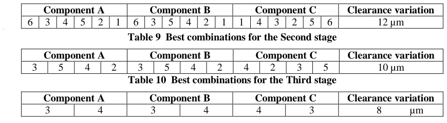
3 5 4 2 3 5 4 2 4 2 3 5 10 µm

Table 10 Best combinations for the Third stage

3 4 3 4 4 3 8 µm

VII. CONCLUSION

The proposed method can be easily implemented in manufacturing. The mating parts are manufactured and they are divided into six groups using snap gauges and kept in separate bins. The best combination is obtained using GA as in the proposed method. In first stage, a component (Part A), a component of (Part B) and a component of (Part C) is taken from the bins as per the best combination and assembled. The best combination in the first stage is used and the components are assembled until the groups 1 and 6 are fully exhausted. Then the best combination in stage 2 is used and the components are assembled until the components in group 2 and 5 are fully exhausted. Then the best combination in stage 3 is used and the components are assembled until the components in groups 3 and 4 are fully exhausted.

The GA, SAA and MA is used for obtaining the best combination of selective groups for minimizing the assembly clearance variation. It is done in three stages to utilize the entire population of mating parts. In the case of the ball bearing assembly with the interchangeable system, the assembly clearance variation of the three components is 42 µm. Whereas the assembly clearance variation using GA is 16 µm for the first stage, 10 µm for the second stage and 8µm for the third stage in SAA is 12 µm for the first stage, 10 µm for the second stage and 8µm for the third stage of the ball bearing assembly. In MA it is 12 µm for the first stage, 10 µm for the second stage and 8µm for the third stage A computer program in ‘C’ language is used to calculate the best combination of selective groups using SAA and MA. From the results to minimize the clearance variation of high precision assemblies either SAA or MA can be used Thus, very high precision assemblies are obtained using the proposed method.

REFERENCES

[1] Allen Pugh, G. (1986) ‘Partitioning for selective assembly’, Computers and Industrial Engineering, Vol. 11, Nos. 1–4, pp.175–179.

[2] Allen Pugh, G. (1992) ‘Selective assembly with components of dissimilar variance’, Computers and Industrial

Engineering, Vol. 23, Nos. 1–4, pp.487–491.

[3] Anand Kumar, M.P.P., Maheswaran, R. and Raj, M.V. (2013) ‘Minimizing clearance variation by

applying genetic algorithm in selective assembly’, Int. J. of Advanced Engineering Applications, Vol. 2, No. 3, pp.92–102.

(8)

[6] Chan, K.C. and Linn, R.J. (1998–1999) ‘A grouping method for selective assembly of parts of dissimilar distributions’, Quality Engineering, Vol. 11, No. 2, pp.221–234.

[7] Coullard, C.R., Gamble, A.B. and Jones, P.C. (1998) ‘Matching problems in selective assembly operations’, Annals of Operations Research, Vol. 76, pp.95–107.

[8] De, T.N., Sundarrajan, S. and Rao, G.K.M. (2013) ‘Optimum size selection for spring loaded

detachable canister launch vehicle interface for multistage long range system’, Int. J. of Engineering Trends and

Technology, Vol. 5, No. 1, pp.1–9.

[9] Desmond, D.J. and Setty, C.A. (1962) ‘Simplification of selective assembly’, Int. J. of Production Research, Vol. 1, No. 3, pp.3–18.

[10] Fang, X.D. and Zhang, Y. (1995) ‘A new algorithm for minimizing the surplus parts in selective assembly’,

Computers and Industrial Engineering, Vol. 28, No. 2, pp.341–350.

[11] Jeevanantham, A.K. and Kannan, S.M. (2013) ‘Selective assembly to minimize clearance variation

in complex assemblies using fuzzy evolutionary programming method’, ARPN Journal of Engineering and Applied

Sciences, Vol. 8, No. 4, pp.280–289.

[12] Kannan, S.M., Asha, A. and Jayabalan, V. (2005) ‘A new method in selective assembly to minimize clearance variation for a radial assembly using genetic algorithm’, Quality Engineering, Vol. 17, No. 4, pp.595–607.

[13] Kannan, S.M., Sivasubramanian, R. and Jayabalan, V. (2009) ‘A new method in selective assembly for components with skewed distributions’, Int. J. Productivity and Quality Management, Vol. 4, Nos. 5/6, pp. 569–589. [14] Lu, C. and Fei, J-F. (2015) ‘An approach to minimizing surplus parts in selective assembly with genetic algorithm’, Proceedings of the Institution of Mechanical Engineers, Part B: J. of Engineering Manufacture, Vol. 229, No. 3, pp.508–520.

[15] Mansoor, E.M. (1961) ‘Selective assembly – its analysis and applications’, Int. J. of Production Research, Vol. 1, No. 1, pp.13–24.