78
Development Of A Modified Wiener Algorithm In
The Restoration Of Digital Images
Oke Alice O, Omidiora Elijah O, Fakolujo Olaosebikan A.
Abstract: Digital image processing has made its way into today’s technology and Computer driven Society with applications encompassing a wide variety of specialized disciplines. Image degradation, however, becomes a serious threat to image processing as current trend in security measures tends towards the use of biometrics. Moreover, data collected using image sensors are generally contaminated by noise and region of interest in the image degraded by many factors among which is motion blur during acquisition, thus, the need to recover or reconstruct the original image. Several image restoration algorithms have been developed to minimize such errors. Wiener filtering algorithm has been and still being adjudged the best restoration algorithm for the clas of linear methods. However, it has the tendency to cause undesirable artifacts in the resultant image. In order to remove the undesirable artifacts, this paper developed a modified Wiener algorithm. Performance of which was evaluated and Computational results showed modified Wiener performed better than the conventional Wiener algorithm.
Index Terms: Convolution, Degradation, Restoration, Simulation, Wiener Algorithm.
————————————————————
1
I
NTRODUCTIONImage processing operates on images and produces images as output, with changes intended to improve the visibility of features or to make the images better for printing or transmis-sion, or to facilitate subsequent analysis. Images are, howev-er, degraded by object or camera motion and noise during image acquisition and this affects the quality of the image. Consequently, it deteriorates the effectiveness of object rec-ognition, event detection and visual perception. Image restora-tion is used to remove or minimize this degradarestora-tion. The key to image restoration is to model the degradation and then to use an inverse operation to reverse it [15]. The recovery of an orig-inal image from degraded observations is of crucial impor-tance and finds application in several scientific areas including medical imaging and diagnosis [7], military [14], surveillance [4], satellite and astronomical imaging [9], and remote sensing [23]. A number of various algorithms have been proposed based on the class of restoration technique. There are eight image restoration techniques, Continuous Image Spatial Filter-ing Restoration is the method for the class of imagFilter-ing systems in which the spatial degradation can be modeled by a linear-shift-invariant impulse response and the noise is additive, res-toration of continuous images can be performed by linear filter-ing techniques [21].
Under this class there is Inverse filtering, Wiener filtering and Parametric estimation filtering methods. The simplex method for reconstructing a degraded image is the use of inverse filter-ing method which inverts the degraded function of the system to yield a restored image [21]. This method will however not produce a perfect reconstruction in the presence of noise. Im-proved restoration quality is possible with Wiener filtering technique because it alleviates noise problem inherent to in-verse method [19]. Wiener filtering method has since been adjudged as the best restoration algorithm for the class of li-near methods under the suitable condition of addictive Gaus-sian noise. Early efforts in the application of Wiener method was geared towards magnetic fields that were contaminated by noise [10], improving signal-to-noise and resolution in acoustic images [20], magnetic profiling in the volcanic envi-ronment of Mt. Etna [5], image and video denoising [19], Ju, Hua, Jiande and Daizhen, [13] combined it with SAR to esti-mate a single high-resolution image from different low-resolution images. However, it has the tendency to cause un-desirable artifacts in the resultant image. Also, Gaussian noise has been the default noise model and suitable condition for Wiener restoration algorithm [24]. Other algorithms such as constraint least square filter and geometric filter have been proposed to remove the undersirable artifacts but whose per-formance either tends to inverse or Wiener filtering method [9]. In this paper, a modified Wiener restoration technique was proposed by hybridizing Constrained least error method and parametric restoration algorithm aimed at reconstruction im-ages that have been degraded by Gaussian noise and linear motion blur. The performance of the modified Wiener restora-tion algorithm was evaluated using quantitative performance measures of root mean square error (RMSE), signal-to-noise ratio (SNR), peak signal-to-noise ratio (PSNR). Computational result showed that modified Wiener performed better than the conventional Wiener algorithm.
2
LINEAR
MOTION
BLUR
Motion blur is an effect you will see in photographs of scenes where objects are moving. It is mostly noticeable when the exposure is long, or if objects in the scene are moving rapidly. Many types of motion blur can be distinguished all of which are due to relative motion between the recording device and the scene. This can be in the form of a translation, a rotation, a sudden change of scale, or some combinations of these [17]. It is defined by the Point Spread Function (PSF) given by (1). ___________________________
A.O.Oke is with the Computer Science and Engineering Department, Ladoke Akintola University of Technology, Ogbomoso, Oyo State. Nigeria.
E.O.Omidiora is with the Computer Science and Engi-neering De-partment, Ladoke Akintola University of Technology, Ogbomoso, Oyo State. Nigeria.
O.A.Fakolujo is with the Electrical and Electronics Engi-neering Department, University of Ibadan, Ibadan, Oyo State, Nigeria.
2.1 Noise Model
Noise is any undesired information that contaminates an im-age. Noise appears in images from variety of sources. The digital image acquisition process, which converts an optical image into a continuous electrical signal that is then sampled, is the primary process by which noise appears in digital im-ages [24]. At every step in the process there are flunctuation caused by natural phenomena that add a random value to the exact brightness value of a pixel. Images are prone to different types of noise some of which are: Gaussian, Salt and Pepper, Speckle, Poisson, Rayleigh, Erlang, Exponential, Uniform, Periodic [15]. Gaussian Noise is the most common and occurs in all recorded images to a certain extent. It is due to the dis-crete nature of radiation that is the fact that each imaging sys-tem is recording an image by counting photons. This noise can be modeled with an independent, additive model, where the noise has a zero-mean Gaussian distribution described by its standard deviation (σ) or variance [14]. This means that each pixel in the noisy image is the sum of the true pixel value and a random, Gaussian distributed noise value. The probability density function is described by (2).
(2)
where 𝝈𝟐= Variance, 𝒙 = is the gray level and 𝝁= mean value.
2.2 Convolution
In mathematics, specifically, functional analysis, convolution is a mathematical operation on two functions f and g, producing a third function that is typically viewed as a modified version of one of the original functions [1]. Linear filtering of an image is accomplished through convolution. Here, convolution is a neighborhood operation in which each output pixel is the weighted sum of neighboring input pixels. The matrix of weights is called the convolution kernel, also known as the filter [25].
3. ANALYTICAL TECHNIQUES
A blurred or degraded image is approximately described by the (3).
(3)
where 𝐹0 𝑥, 𝑦 is the degraded (blurred and noisy) image, 𝐹1 𝑥, 𝑦 is the original image, which represents the image ob-tain under a perfect image acquisition condition, in this case the input image. 𝐻𝐷 𝑥, 𝑦 is the distortion operator, also called the PSF. When the distortion operator is convolved with the image, it creates the distortion. 𝑁 𝑥, 𝑦 is the additive noise which is introduced during image acquisition, that corrupts the image [21], [16]. After restoration with this filter, the recon-structed image is represented by the (4).
(4)
Where 𝐹 1 𝑥, 𝑦 is the restored image, 𝐹0 𝑥, 𝑦 is the degraded image and 𝐻𝑅 𝑥, 𝑦 is the restoration filter. From (3) and (4).
(5)
Fig1.ps shows a typical image restoration model, giving (3) and (4) in graphical form. This technique was applied to dis-crete images, each of the spectral functions involved in the filtering operation was replaced by its discrete two dimensional Fourier transform counterpart of (6). Fourier transform is im-portant because convolution in spatial domain and multiplica-tion in frequency domain constitutes a Fourier transform pair. Hence, (5) in the Fourier transform has the advantage of short computation time to produce solution [9].
(6)
where ℱ 1 𝜔𝓍, 𝜔𝓎 , ℱ1 𝜔𝓍, 𝜔𝓎 , ℋ𝐷 𝜔𝓍, 𝜔𝓎 , 𝒩 𝜔𝓍, 𝜔𝓎 and ℋ𝑅 𝜔𝓍, 𝜔𝓎 are the two-dimensional Fourier transforms of 𝐹 1 𝑥, 𝑦 , 𝐹1 𝑥, 𝑦 , 𝐻𝐷 𝑥, 𝑦 , 𝑁 𝑥, 𝑦 and 𝐻𝑅 𝑥, 𝑦 respectively.
Fig.1. Image Restoration Model
3.1 Inverse Filtering Method
Inverse filtering concept inverts the PSF of the degrading sys-tem to yield a restored image [3], [19], [21]. The restoration inverse filterPSF is chosen so that
(7)
then the spectrum of the reconstructed image becomes
(8)
Inverse filtering will however not produce a perfect reconstruc-tion in the presence of noise but if source noise is present, there will be an additive reconstruction error whose value can become quite large at spatial frequencies for which ℋ𝐷 𝜔𝓍, 𝜔𝓎 is small [6]. Another fundamental difficulty with inverse filtering is that the transfer function of the degradation may have zeros in its passband, which makes the inverse filter not physically realizable, and therefore the filter must be ap-proximated by a large value response at such points.
3.2 Constrained Least-square Error Filter
Constrained least-square error filter and Parametric filter [6] were proposed in a bid to further alleviate noise. Taking into account the noise influence on inverse filter, a linear function of the estimated image can be minimized under a constraint [11] related to the noise as (9)
(9)
With
80 The restoring filter in Fourier transform is (11), [17], [21].
(11)
Where 𝛾 is adjusted to satisfy Equation (10). 𝛾 in (11) is a de-sign constant and 𝐿 𝜔𝑥, 𝜔𝑦 is a design spectral variable. If 𝛾
= 1 and 𝐿 𝜔𝑥, 𝜔𝑦 2
are set equal to the spectral ratio of Wiener Equation, ―Equation (11) becomes equivalent to the Wiener filter‖. If there is no blurring of the ideal image, ℋ𝐷 𝜔𝑥, 𝜔𝑦 = 1, the Wiener filter becomes the inverse filter. One of the various choices that have also been proposed for 𝐿 𝑥, 𝑦 is (12) and the restoration filter is (13), [6].
(12)
(13)
This filter tries to minimize the energy of the gradient of the estimated image, it thus limits the effect of the noise. This mi-nimization of the energy of the restored image is weighted by the confidence reposed in the restored image. This confidence is measured through the signal to noise ratio. When 𝛾 varies from 0 to 1 this filter varies from the inverse filter to the Wiener filter [6].
3.3 Parametric Filter
Another approach is in forcing the spectrum of the restored image to be equal to the spectrum of the input image
(14)
Thus
(15)
Where 𝑆𝐹2 in (14) equals 𝐻𝐷 𝑥, 𝑦 2𝑆𝐹1 𝑥, 𝑦 + 𝑆𝑁 𝑥, 𝑦 in (15).
Enforcing this spectrum to be equal to 𝑆𝐹1 𝑥, 𝑦 leads to the
restoration filter of (16) in the Fourier transform [6], [2].
(16)
Equation (16) takes into consideration the geometric mean between the inverse and the Wiener filter. Equation (17) is the generalized form of (16).
(17)
Equations (13) and (16) are termed parametric filters, they are
seen as variant of Wiener filter. Though these filters are found to be good but have not measured to the performance of Wiener filtering in restoration. Their performance either tend to Inverse or Wiener filter [21].
3.4 Wiener Filter
Improved restoration quality is possible with Wiener filtering techniques, because it alleviates noise problems inherent to inverse filtering by incorporating apriori statistical knowledge of the noise field [21]. The Wiener filter is a linear spatially invariant filter of the form of (3). Its PSF, ℋ𝐷 𝜔𝓍, 𝜔𝓎 is chosen such that it minimizes the mean-square restoration error (MSE) between the input and the restored image. This crite-rion attempts to make the difference between the original im-age and the restored one, that is, the remaining restoration error which should be as small as possible on the average:
(18)
The solution of the minimization problem of (18) is known as the Wiener filter, and is defined as:
(19)
where 𝐻𝐷∗ 𝑥, 𝑦 is the complex conjugate of 𝐻𝐷 𝑥, 𝑦 , 𝑆𝑁 𝑥, 𝑦 is the power spectrum of the noise, 𝑆𝐹1 𝑥, 𝑦 is the power spectrum of the input and 𝐻𝑅 𝑥, 𝑦 is as previously defined. This filter is convolved with the degraded image to give a res-tored image [8]. The power spectrum is a measure for the av-erage signal power per spatial frequency 𝑥, 𝑦 carried by the image. The noise is assumed to be uncorrelated, so its power spectrum is determined by the noise variance only given in (23), [17].
(20)
The power spectrum of the input image is estimated from the power spectrum of the degraded image and compensated for the variance of the noise, this is given as (21).
(21)
3.5 Modified Wiener Filtering Model
The Constrained least-square error filter yields a smoother restoration but its deblurring is not as effective as that of Wiener technique [18]. Parametric filter performance tend to-wards Wiener’s and due to the undesirable artifacts in the re-sultant image produced from Wiener technique, a need arises to modify Wiener in order to further minimize the error and improve on the resultant image [24]. Equation (22) is the hy-bridization of constrained least-square error and the parame-tric filters. Hence, the advantage of the smoother restoration of the constrained least-square error filter and the property of the parametric filter with 𝛼 and 𝛾 as the two tuning parameters [6] were combined to arrive at (25).
Let
(23)
Therefore
(24) Hence
(25)
4. MATERIALS AND METHOD
The proposed algorithm was carried out on a Compaq Presa-rio CQ60 notebook PC with typical specification of an AMD Athlon Dual-Core QL-62 GHz processor board, 32-bit Window Vista operating system and 2.00GB Ram using Image processing tools of MATLAB (version 7.9.0.529 (R2009b)). The first phase was the acquisition of data, which is achieved by making use of direct imaging system. A Canon Powershot SD400 was the digital camera (with effective pixels of approx-imately 5.0 million, image sensor of ½.5-inch CCD and lens of 5.8 (W) – 17.4 (T) mm)used for the parallel acquisition tagged real while Photosmart 330 scanner was used for serial acquisi-tion tagged scanned. Samples of various sizes were collected through the two sources. The data obtained from the sampled image was required in the modelling of the degradation. Simu-lation of the linear motion blur was first carried out using (1). Linear motion blur was employed because the restoration sys-tem being considered is of a linear-shift-invariant filter defined by the impulse response. This process was performed by creating a PSF that simulated the blur which is required to degrade the image. The blur was implemented by first creating a PSF filter which approximates the linear motion blur. This PSF was then convolved with the input image and the blurred image was produced. The amount of blur generated is a func-tion of the length of the blur (in pixels) and the angle of the blur. These parameters were altered to generate variations of blur, and ultimately a length of 31 pixels at an angle of 11 de-grees were found to generate sufficient motion blur to the im-age. Gaussian noise was introduced to the blurred image and the developed restoration algorithm was then applied on the degraded image 𝛾 being varied. This was convolved with the blurred and noisy image to remove the blur and noise, the op-timum restoration was found at 𝛾 = 0.95. The performance of the developed restoration algorithm was evaluated based on three statistical measurements, RMSE, SNR and PSNR ―[26]‖. These parameters were used to determine the rate of restora-tion with the noise variance varied from 0.0001 to 0.01. Re-sults from restoration with the developed algorithm were eva-luated with Wiener algorithm. Restoration of blurred and noisy images acquired from parallel acquisition was also compared with that of serial acquisition. The SNR of the blurred and noi-sy image is defined as follows in decibels:
(26)
The improvement in SNR is basically a measure that ex-presses the reduction of disagreement with the input image when evaluating the distorted and restored image. The Mean Square Error (MSE) is the average error per pixel and the RMSE is the square root of the MSE. ―Equation (27) indicates the formula for RMSE‖.
(27)
(28)
5. RESULTS AND DISCUSSION
An appreciable removal of the noise and blur was observed when the modified Wiener algorithm was applied to the de-graded image. However, it was not possible to obtain perfect reconstruction because ideal image is not usually available in practice that would have provided the properties for correct measurement [22], as presented under Wiener algorithm. Fig2.ps to fig4.ps represent the graph of RMSE, SNR and PSNR respectively against variance for the restoration of real degraded image for Wiener and Modified Wiener algorithms. In Fig2.ps, Modified Wiener has lower values of RMSE com-pared with that of Wiener algorithm for all values of the va-riance considered. This shows an improvement of Modified Wiener algorithm over Wiener. The least value of RMSE was found at variance value 0.0002 for both Wiener and modified Wiener. This is in contrast to 0.0001 found in [22]. This implies that the error in variance value 0.0001 is not the least, that the system was discovered to have higher noise immunity. Fig3.ps and fig4.ps showed modified Wiener having higher SNR and PSNR than Wiener algorithm for all values of variance consi-dered except at 0.0009 where both algorithms have the same PSNR according to the experiment carried out which is as shown in Fig4.ps. The highest SNR value on fig3.ps coincided with variance value 0.01 inspite of the large RMSE. Indicating that there can be a tradeoff between SNR and RMSE. With a lower RMSE and higher SNR and PSNR, the graph showed that modified Wiener has a better performance than Wiener algorithm. Fig5.ps to fig7.ps represents the graph of RMSE, SNR and PSNR respectively against variance for the restora-tion of Scanned degraded image using Wiener and Modified Wiener. The results revealed exhibition of similar characteris-tics to real images with real images giving higher absolute val-ue than the scanned images.
82 Fig.3. SNR against Variance for Real degraded image with
Gaussian Noise
Fig.4. PSNR against Variance for Real degraded image with Gaussian Noise
Fig.5. RMSE against Variance for Scanned degraded image with Gaussian Noise
Fig.6. SNR against Variance for Scanned degraded image With Gaussian Noise
Fig.7. PSNR against Variance for Scanned degraded image with Gaussian Noise
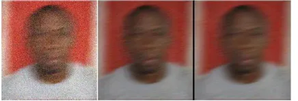
Plates 1 and 2 show selected pictorial view of the results of real and scanned Image respectively. Each shows the real and scanned, blurred Noisy image, Wiener algorithm and Modified Wiener algorithms implementation respectively. Modified Wiener algorithm gave a better picture quality than Wiener for all the variance values shown. The significant change is not so much visible, this is because the differential change can only be measured by the system through the statistical measure-ments which has already been given by the fig2.ps to fig7.ps above.
(a) Real, Noisy blurred with Var = 0.0001, (b) Wiener algorithm (c) Modified Wiener algorithm
(a) Real, Noisy blurred with Var = 0.0002, (b) Wiener algorithm (c) Modified Wiener algorithm
(a) Real, Noisy blurred with Var = 0.01, (b) Wiener algorithm (c) Modified Wiener algorithm
Plate 1. Pictorial analysis of the algorithms using real image
(a) Scanned, Noisy blurred with Var = 0.0001, (b) Wiener algorithm (c) Modified Wiener algorithm
(a) Scanned, Noisy blurred with Var = 0.0002, (b) Wiener algorithm (c) Modified Wiener algorithm
(a) Scanned, Noisy blurred with Var = 0.008, (b) Wiener algorithm (c) Modified Wiener algorithm
(a) Scanned, Noisy blurred with Var = 0.01, (b) Wiener algorithm (c) Modified Wiener algorithm
Plate 2. Pictorial analysis of the algorithms using Scanned image.
Table 1 evaluates the overall performance of restoration for both Real and Scanned image samples between Wiener and Modified Wiener, showing that Modified Wiener is better. Mod-ified Wiener is more efficient than Wiener with the variance values classified as low (0.0001 - 0.0009) and high (0.001 - 0.01) for all the parameters considered.
Table1. Summary of Results of Better Restoration between Wiener and Modified Wiener for Real and Scanned images
6. CONCLUSION
In this work, the developed algorithm was obtained by hybri-dized Constrained least error method and parametric restora-tion algorithm for the reconstrucrestora-tion of images degraded by Gaussian noise and linear motion blur. This is in order to re-move the artifact which is common with Wiener restoration technique and improve signal quality. Samples of images from two imaging systems: parallel and serial acquisitions were considered. The degradation was simulated employing the linear motion blur and Gaussian noise models. The modified Wiener algorithm was applied to restore each degraded im-age. The performance of this algorithm was evaluated using quantitative performance measures of RMSE, SNR and PSNR with a range of noise variance, as well as in terms of visual quality of the images. The noise variance was tested for values 0.0001 to 0.01 and greater values than 0.01 in steps of 0.05 to 1.0. A similar trend of the given result ensued but litera-ture has a stable variance value of 0.0001, that accounted for the choice range of 0.0001 to 0.01. Using RMSE and SNR as the objective measurements, the least error value and highest SNR value were found to be at variance values 0.0002 and 0.01 respectively. There arises a tradeoff between the RMSE and SNR since the values do not coincide. This means that if signal is the focus, it will be at the expense of the error. The performance was evaluated with standard Wiener algorithm. Computational results showed that modified Wiener algorithm performed optimally well in the restoration of the degraded images for both low and high noise variance values. Further-more, the results showed that quality of the restored image from parallel acquisition was better with lower values of RMSE and higher values of SNR than the serial acquisition. The main reason for this could be attributed to the acquisition method employed.
ACKNOWLEDGEMENTS
84
R
EFERENCES[1] Bracewell, R. (1986). The Fourier Transform and Its Applications (2nd ed.), McGraw– Hill, New York.
[2] Brigo, D., Hanzon, B., François L. (1998). A Differen-tial Geome- tric approach to nonlinear filtering: the Projection Filter, IEEE Transactions on Automatic Control. 43 (2): 247--252.
[3] Chang S.G., Bin Y., Vetterli M. (2006). Adaptive wave-let thres-holding for image denoising and compres-sion, IEEE Trans. On Image Processing, 9 (9): 1532-1546.
[4] Chung-Hao C., et al (2008). Surveillance Systems with Automa-tic Restoration of Linear Motion and Out-of-focus Blurred Images. ICIC Express Letters. 2(4): 409-414.
[5] Del Negro (1996). Application of the Weiner filter to Magnetic Profiling in the Volcanic Environment of Mt. Etna (Italy), Annali Di Geofiscia, XXXIX(1): 67-79.
[6] Faugeras, O. D. (1983). Fundamentals in Computer Vision: Press Syndicate of the University of Cam-bridge, USA.
[7] Geoff D. (2009). Digital Image Processing for Medical Applica-tions, Cambridge University Press, New Del-hi, India.
[8] Gonzalez R. C., Woods R. E., Eddins, S. L. (2004). Digital Image Processing Using MATLAB, 2nd edition, Gatesmark Publishing, Knoxville.
[9] Gonzalez R. C., Woods R. E. (2007). Digital Image Processing, 3rd edition, Pearson Prentice Hall.
[10]Gunn, P. J. (1975). Applications of Wiener filters to remove Au tocorrelated Noise from Magnetic Fields, Bulletin of the Aus-tralian Society of Exploration Geo-physicists 5(4): 127-130.
[11]Hunt, B.R. (1973). The Application of Constrained Least Square Estimation to Image Restoration by Digital Computer, IEEE Transactions on Computers, 2: 805-812.
[12]Hykes D, et al (1985). Ultrasound Physics and In-strumentation, Churchill, Livingstone Inc., New York.
[13]Ju L., et al (2003): ―Super-Resolution Image Restora-tion by Combining Incremental Wiener Filter and Space-Adaptive Re-gularization, IEEE International Conference Neural Networks & Signal Processing, 998-1001.
[14]Katsaggelos, A. K. (1991). Digital Image Restoration, Springer Verlag, New York.
[15]Kenneth R. C. (1996). Digital Image Processing: Prentice-Hall Inc., New Jersey.
[16]Lagendijk, R., Biemond, J. (1991). Iterative Identifica-tion and RestoraIdentifica-tion of Images, Kluwer Academy Publishers, Boston, M.A.
[17]Lagendijk R., Jan B. (1999). Basic Methods for Image Restora- tion and Identification‖ in Handbook of Image and Video Processing, ed. Al Bovik. New York.
[18] Ling G., Rahab K. W. (1990). Restoration of Stochastically blurred images by the Geometrical Mean Filter, Optical Engineering, 29(4): 289-295.
[19] Liu, J. J. (1997). Applications of Wiener Filtering in Image and Video De-noising, ECE497KJ Course project, 1-15.
[20]Mitchell, K. W., Gilmore, R. S. (1991): ―A true Wiener Filter Im plementation for Improving Signal to Noise and Resolution in Acoustic Images’, Proceedings of the 18th Annual Review, Brunswick, ME, 11A: 895-902.
[21]Pratt, W. K. (2007). Digital Image Processing, 2nd edition, Wi ley, New York.
[22]Rafael, C. G., Richard, E. W., Steven, L. E. (2003). Digital Image Processing Using MATLAB, Prentice Hall Publication, New Jersey.
[23]Ram M. N., Sudhir K. P., Stephen E. R. (2001). Ef-fects of Uncor related and Correlated Noise on Image Information Content‖, Geoscience and Remote Sens-ing Symposium, IGARSS, IEEE 2001, 4: 1898-1900
[24]Scott E. U. ( 1998). Computer Vision and Image Processing, Prentice Hall PTR, New Jersey,
[25]Smith, J. O. (2007). Introduction to Digital Filters with audio Application, Center for Computer Research in Music and Acoustics (CCRMA), Stanford University.
[26]Thangavel, K., Manavalan, I., Aroquiaraj, I. L. (2009). Removal of Speckle Noise from Ultrasound Medical Image based on Special Filters: Comparative Study. ICGST-GVIP Journal,9, (III).
Oke A. O., has B.Tech (Hons) Computer Engineering, (1998), M.Tech Computer Science, (2005), Ph.D Computer Science, (2012); Ladoke Akintola University of Technology, Ogbomoso, Oyo State, Nigeria. Working in the same institution, 2001 till date; 31 paper publications in Journals, conference proceed-ings and as books.research interest includes: Image processing algorithms, Compression algorithms and hardware design and implementation. She is a Registered Engineer, The Council for Regulation of Engineering in Nigeria (COREN) and member Computer Professional (Registration) Council of Nigerian (MCPN).
working in Ladoke Akintola University of Technology, Ogbomo-so, Nigeria. Presently, he is the Head of Depart of Computer Engineering, Federal University, Oye-Ekiti, Nigeria, where he is spending his sabbatical leave. He has over 90 publications in reputable Journals and conferences. His research interest include:the study of Biometric systems and Biometric-based Algorithms and its applications to Security issues in systems, Computations Complexity measures and soft computing. He is a member of Computer Professional (Registration) Council of Nigerian (MCPN), a Registered Engineer, Council for Regula-tion of Engineering in Nigeria (COREN) and Corporate mem-ber, Nigerian Society of Engineers.