Modelling Software Reliability Growth Phenomenon In Distributed Development Environment

2176

Modelling Software Reliability Growth Phenomenon

In Distributed Development Environment

Nesreen Qallab, Omar Shatnawi

Abstract: The present scenario of software development life-cycle has switched into a distributed environment because of the development of network technology and ever increased demand of sharing the resources to optimize the cost. In the software reliability engineering literature, few attempts have been made to model the fault testing and debugging process in a distributed development environment. One of the reasons can be attributed to the complexity involved in developing large-scale distributed systems. As a result, their testing and debugging process is influenced by many internal and external factors, all of which may not be deterministic in nature. Since reliability is the only measure of software quality, a software reliability model is needed to estimate the current reliability level and the time and resources required to achieve the objective reliability level. As the area of software fault-debugging in distributed development environment is not thoroughly investigated in current literature, even though it is estimated to have been one of the most expensive endeavor in the industry. This objective dictates developing a non-homogenous Poisson Process based testing-effort dependent software-reliability modelling approach for distributed-systems developed under imperfect-debugging environment. The resultant integrated modelling approach describes the relationship among the calendar time, the testing-effort consumption, and fault- correction/debugging process under imperfect-debugging environment. To the best of our knowledge this is the first time that this kind of integration modelling approach has been carried out for distributed systems. Fault-debugging process and testing-effort expenditures are described by a non-homogenous Poisson process and testing-effort curve functions respectively. Such a type of integrated modelling approach is very much suited also for object-oriented software development. Actual software reliability data cited in literature have been employed to demonstrate the applicability of the proposed integrated modelling approach. The results are fairly encouraging when compared with other existing approaches developed under similar environment.

Index Terms: Software Reliability Engineering, Distributed Development Environment, Software Testing and Debugging, Non-Homogenous Poisson Process, Imperfect Fault Debugging, Error Generation, Fault Debugging Complexity.

——————————  ——————————

1

I

NTRODUCTION

Developing large-scale distributed software system is generally a quite complex and time consuming process. Due to their development complexity, these systems are hardly ever ―perfect‖ [1]. However, the nature and complexity of their requirements have drastically changed and users all over the world have become much more demanding in terms of cost, schedule and quality. Several techniques available for studying the cost and schedule of software; however, reliability is the only measure of software quality [2]. As software is created by error-prone humans, and there is no way to prevent programmers from making mistakes. Faults can be introduced during the software development lifecycle. Therefore, it is impossible to guarantee a failure-free software system [3], [4], [5], [6], [7], and [8]. In software reliability engineering literature, fault-debugging is challenging, and least developed. Software fault-debugging process is the process of detecting, locating, and correcting faults in software [9]. Approximately 20% of all software faults take 80% of all the required effort to debugging software faults [10]. Software failure is estimated to cost American industries USD 60 billion every year [11]. Jones state that imperfect-debugging of faults were discovered in almost every company [12]. Reusability is a key direction to improving software development productivity and quality, as it entails all entities of software development life cycle [13]. Due to high demand on quality and productivity in social systems, measuring software reliability in distributed development environment is major concern for software developers [5], [13], [14], and [15].

Software testing-effort expenditure is measured by resources such as man power spent during testing, CPU hours, number of test cases etc. Musa [2] indicated that the testing effort index or the execution time is a better time-domain for software reliability modeling than the calendar time. About half of the resources consumed during the software development cycle are testing resources. These testing resources spent in testing appreciably affect software reliability. The consumption curve of these resources over the testing period can be thought of a testing-effort curve. In other words, the function that describes how testing resources are distributed is usually referred to as testing-effort function and it has been incorporated into software reliability modelling. Various forms of testing-effort functions have been used in the literature viz., exponential, Rayleigh, Weibull, logistic etc. to represent effort consumption [16], [17], [18], [19], [20], and [21]. The rest of the paper is organized as follows: Section 2 reviews some of the well-documented and established non-homogenous Poisson process (NHPP) based software reliability model for software quality/reliability measurement and assessment in a distributed development environment. Section 3 proposes a newly developed quantitative technique for software quality/reliability measurement and assessment model. Section 4 defines the technique that has been employed for parameter estimation and software reliability data analyses, and provides the comparison criteria used for validation and evaluation. Section 5 presents the applications of the proposed integrated modelling approach to actual software reliability data through data analyses and model comparisons. Section 6 concludes and identifies possible avenues for future research.

2

S

OFTWARE

R

ELIABILITY

M

ODELLING IN

D

ISTRIBUTED

D

EVELOPMENT

E

NVIRONMENT

:

L

ITERATURE

R

EVIEW Software reliability models are useful in measuring reliability for the quality control and testing process control of software development. Many models have been proposed, but a few of

————————————————

• Nesreen Qallab, Computer Science Department, Al al-Bayt University, Jordan.

2177 them have actually been applied to several software

management tools which aid the software quality or reliability measurement and testing–progress control [5], [7], [22], [23], and [24]. Nowadays, NHPP models contribute to software reliability measurement in many software development houses [6], and [25]. They consider the debugging process as a counting process characterized by the value function of NHPP. Software reliability can be estimated once the mean value function is determined. Model parameters are usually determined using either maximum likelihood estimation (MLE) or least-square estimation (LSE) methods [5], [7], [26], and [27].

2.1 Software Reliability Modelling

The software development environment is changing from a host-concentrated one to a distributed one due to cost and quality aspects and rapid growth in network computing technologies. Under this environment software component can be developed at different geographical locations and components used in other software can be re-used. The NHPP based models that explain the software reliability growth phenomenon in distributed development environment can be classified into two categories. The first category is time-dependent behavior of fault correction process, that is, the number of software faults being corrected is proportional to the remaining number of faults [14]. The second category is time-dependent variation in testing-effort consumption, that is, the number of software faults being corrected by the current testing-effort expenditures at any time is proportional to the remaining number of faults [15]. Some of the general assumptions (apart from some special ones for specific models discussed) assumed in the models are as follows:

 Fault removal or debugging process follows NHPP. For re-used and newly-developed components has been modelled individually and is summed up to get the total removal or debugging process of the software system

 Software is subject to failure during execution at random times caused by the manifestation of remaining faults.

 Software reliability growth phenomenon in the re-used components is uniform (i.e., follows an exponential growth curve) while in the newly-developed component is not (i.e., follows an S-shaped growth curve).

The following are some of NHPP based software reliability growth models that proposed for distributed development environment.

2.1.1 Yamada et al. [14] Model

This model was a pioneering attempt in the field of software reliability modeling and paved the way for modelling software reliability in distributed development environment. In this model, the authors claimed that it is empirically well-known that the cumulative number of detected faults follows an exponential curve when a software system consisting of several used components are tested in the testing phase; while on the other hand, the cumulative number of faults is described by an S-shaped growth curve when the newly developed component is used. Accordingly, they constructed a software reliability model for software systems developed under such an environment, which incorporates the delayed S-shaped model [26] for reused components, and the exponential software reliability model [27] for newly developed components.

2.1.2 Shatnawi [15] Model

The model integrates testing-effort function into Yamada et al. [14] model to get a better description of the software fault-correction process. To relax the pre-specified fault content-weight or testing-content-weight parameters for each software component that has been adopted in the aforementioned models. The author assumed that he ratio of fault-density and the amount of testing-effort expenditure in re-used to newly-developed component s is about 1 to 4, as reported [28] ―the defect rate for reused code is 0.9 defects per KLOC, while the rate for newly developed software is 4.1 defects per KLOC in a study conducted at Hewlett-Packard (HP)‖.

2.2 Study Motivation

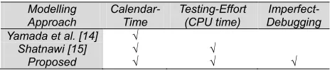
The aforementioned software reliability models are constructed considering the debugging scenarios as tabulated in the below Table 1. However, none of them provide insightful interpretations for both the testing-effort expenditure and imperfect-debugging phenomena during testing and debugging phase. A proposed solution is developing an integrated modelling approach. This necessitates a modelling approach that can be modified without unnecessarily increasing the complexity of the resultant model.

Therefore, this study has attempted to develop an integrated modelling approach, so as to incorporate the effect of fault- correction/debugging complexity with time-dependent variation in testing-effort consumption for distributed systems developed under imperfect debugging environments. Such a type of integrated modelling approach is very much suited also for object-oriented (OO). Experimentation has shown that models based on execution time are superior to those based on calendar-time [2] and [29].

Table 1.

Modelling Approach

Calendar-Time

Testing-Effort (CPU time)

Imperfect-Debugging Yamada et al. [14] √

Shatnawi [15] √ √

Proposed √ √ √

To the best of our knowledge this is the first time that this kind of non-homogenous Poisson process based integration modelling approach that describes the relationship among the calendar time, the testing-effort consumption, and fault- correction/debugging process under imperfect-debugging environment, has been studied for distributed systems.

3 T

ESTING

-E

FFORT

D

EPENDENT

S

OFTWARE

R

ELIABILITY

M

ODELLING FOR

D

ISTRIBUTED

S

YSTEMS IN

I

MPERFECT

D

EBUGGING

E

NVIRONMENT

:

A

P

ROPOSED

I

NTEGRATED

A

PPROACH

3.1 Testing-Effort Modelling

2178 utilization of limited testing resource has become even more

important than before [31]. Software testing-effort expenditure is measured by resources such as man power spent during testing, CPU hours, number of test cases etc. These testing resources spent in testing appreciably affect software reliability. The consumption curve of these resources over the testing period can be thought of a testing-effort curve. Various forms of testing-effort functions have been used in the literature such as exponential, Rayleigh, Weibull, logistic etc. [16], [17], [18], [19], [20], and [21]. To study the testing-effort consumption process, one of the below functions can be selected for the purpose:

 Exponential

 Rayleigh

 Weibull

 Logistic

The first two can be derived from the assumption that, ―the testing effort rate is proportional to the testing resources available.‖

𝑊 = 𝑐(𝑡) ∙ (𝛼 − 𝑊) (1)

Solving (1) under initial condition 𝑊 = 0, yields

𝑊 = 𝛼 ∙ (1 − exp⁡(∫ 𝑐(𝑥) ∙ 𝑑𝑥)) (2)

Case 1: If 𝑐(𝑡) = 𝑐, we get exponential curve:

𝑊 = 𝛼 ∙ (1 − exp⁡(−𝑐 ∙ 𝑡)) (3)

Case 2: If 𝑐(𝑡) = 𝑐 ∙ 𝑡, we get Rayleigh type curve:

𝑊 = 𝛼 ∙ (1 − exp⁡(− ∙ ₎₎ (4)

Case 3: If 𝑐(𝑡) = 𝑐 ∙ 𝑟 ∙ 𝑡 _{, we get Weibull function:}

𝑊 = 𝛼 ∙ (1 − exp⁡(−𝑐 ∙ 𝑡 )) (5) Exponential and Rayleigh curves become special cases of the Weibull curve for 𝑟 = 1 and 𝑟 = 2 respectively.

Case 4: If we define

𝑊 = 𝑐 ∙ (𝛼 − 𝑊) (6)

On solving, the cumulative testing effort consumed in the interval⁡(0, 𝑡) is given by

𝑊 = _{∙ ⁡( ∙ )} (7)

This is the Logistic testing-effort function.

3.2 Integrating Modelling Approach

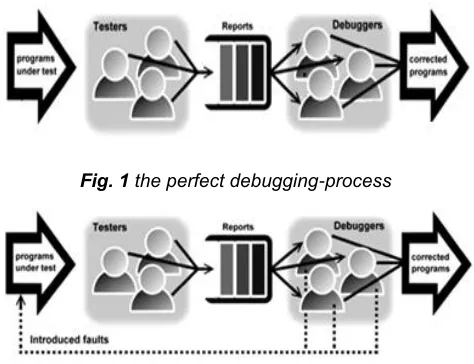
The present scenario of software development lifecycle has emerged into a distributed environment because of the development of network technology and ever increased demand of sharing the resources to optimize the cost. Therefore, distributed systems are fast-growing in reply to the achievements of computer hardware and software industries. Large-scale distributed systems developments are now common in air traffic-control, telecommunications, defense and space [5]. Thus, it is important to assess the reliability of software developed in distributed environment because of increasing the demands on quality and productivity in social systems [13]. Reusability is a key direction to improving software development productivity and quality [16]. Distributed systems are depending heavily on traditional software engineering methodologies [15]. Debugging is one of the most challenging, and least developed areas of software engineering. The testing and debugging activities in perfect

and imperfect debugging environments [32] are depicted in Figures 1 and 2 respectively.

Fig. 1 the perfect debugging-process

Fig. 2 the imperfect debugging-process

The main objective of this study is to develop a software reliability model based on more realistic assumptions depicting different phenomena during the testing and debugging phase in a distributed development environment. The first step in achieving this objective is to identify the unrealistic assumptions which existing models are based on. The second step is to build flexible model which relax these assumptions. The following are some of unrealistic assumptions

 All faults are of the same type, complexity and have the same impact on the reliability growth.

 Testing-effort employed to detect, isolate and correct the faults has the same consumption pattern.

 Pre-specified testing-weight parameters for each software component.

To address these unrealistic issues, a newly developed NHPP based software reliability growth model for distributed system, through an integrated modelling approach incorporating software fault debugging complexity under imperfect fault debugging environment is proposed.

3.2.1 Assumptions and Notations

The following are the basic assumptions in developing the proposed modelling approach:

 Software is subject to failures during execution caused by the remaining faults.

 Fault correction phenomena follows an NHPP with 𝑚 .

 Testing resource is not constantly allocated during software testing phase, which can largely influence the debugging process.

 Faults encountered are of three types: easy, hard, and complex, which are of different debugging complexity.

 The ratio of fault density and the amount of testing-effort expenditure in reused to newly developed components is about 1 to 4.

 Each time a fault is reported, an immediate (delayed) effort takes place to locate/isolate it in order to correct it. The time-delay between the fault detection or located and its subsequent correction is assumed to represent the debugging complexity of the faults.

2179 testing and debugging team may not be able to remove

the fault perfectly and the original fault may remain or get replaced by another fault. While the first phenomenon is known as imperfect debugging, the second is called error-generation.

The following notations are used for the mathematical formulation purpose:

𝑚 Expected number of faults debugged in time-dependent variation in testing-effort consumption (0, 𝑊]

𝑖, 𝑗 Subscripts that denotes the re-used and newly

developed components respectively

𝑚 Expected number of faults debugged in reused components

𝑚 Expected number of faults debugged in newly developed components

𝑊 Amount of testing-effort consumed in the time interval (0, 𝑡]

𝑊 , Expected effort spent on components debugging

𝑊 = 𝑊 ∙ 𝑔; 𝑊 = 𝑊 ∙ 𝑔

𝑤 , Current effort spent on components debugging, that is, 𝑊 = ∫ 𝑤 ∙ 𝑑𝑥

𝑔 , Proportion of effort spent on components debugging 0 ≤ 𝑔(𝑔) ≤ 0.2(0.8); ∑ 𝑔 , = 1

𝑎 Total number of faults lying dormant in software ∑ 𝑎 , = 𝑎

𝑎 , Initial fault-content in components⁡𝑎 = 𝑎ℎ; 𝑎 = 𝑎ℎ

ℎ , Proportion of fault-content in components 0 ≤ ℎ(ℎ) ≤ 0.2(0.8); ∑ ℎ , = 1

𝑝 Probability of fault removal on a detection of a fault 𝛼 Rate at which faults may be introduced during the

debugging process

𝑐 Time dependent rate at which resources are consumed, with respect to remaining available resources

𝛾, 𝑐, 𝑟 Constant parameter in testing-effort functions

3.2.2 Modelling the Imperfect Fault Debugging Process of ‗i‘ Reused Components

To model the fault correction process of ‗i‘ re-used components, the imperfect-debugging model with testing-effort [5] and [19] is adopted for the purpose. The adopted model assumed that reported faults are of type ‗easy to debug‘, and their debugging process is modeled as one-stage process. That is, once the fault is reported it is corrected immediately without delay as illustrated in Figure 3. The model is given as

𝑚 = ∙ (1 − 𝑒 ∙ ∙( )∙ ₎ (8)

The above mean value function in (8) represents the expected number of faults corrected.

Fig. 3 the fault debugging process for ‘easy to debug’ type

3.2.3 Modelling the Imperfect Fault Debugging Process of

‘j’ Newly Developed Components

To model the fault correction process of ‗j‘ newly developed components, the imperfect-debugging model with testing-effort [5] and [19] is adopted for the purpose. The adopted model assumed that reported faults are of two types: ‗hard to debug‘ and ‗complex to debug‘, and their debugging process is modeled as two-stage process and three-stage process receptively. For ‗hard to debug‘ faults, the imperfect debugging process is modeled as a two-stage process—fault detection followed by correction as illustrated in Figure 4. The mean value function for components containing ‗hard to debug‘ faults with boundary condition that 𝑚 = 0 is given as

𝑚 = ∙ (1 − ((1 + 𝑏 ∙ 𝑤 ) ∙ 𝑒 ∙ ₎ ∙( )₎ (9)

Fig. 4 the fault debugging process for ‘hard to debug’ type

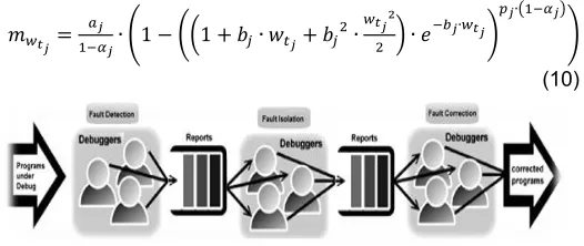
For ‗complex to debug‘ faults, the imperfect debugging process is modeled as a three-stage process—fault detection, isolation followed by correction as illustrated in Figure 5. The mean value function for components containing ‗complex to debug ‗ faults with boundary condition that 𝑚 = 0 is given as

𝑚 = ∙ (1 − ((1 + 𝑏 ∙ 𝑤 + 𝑏 ∙ ) ∙ 𝑒 ∙ ₎ ∙( )

)

(10)

Fig. 5 the fault debugging process for ‘complex to debug’ type

The total imperfect debugging of ‗j‘ newly developed components is the superposition of the sum of the two debugging-process with mean value functions given in (9) and (10) respectively, as

𝑚 = ∙ (1 − ((1 + 𝑏 ∙ 𝑤 ) ∙ 𝑒

∙

) ∙( ))⁡+

∙ (1 − ((1 + 𝑏 ∙ 𝑤 + 𝑏 ∙

_{) ∙ 𝑒} ∙ )

∙( ) )

(11)

3.2.4 Modelling the Total Imperfect Fault Debugging Process

2180 components with mean value functions given in (8) and (11)

respectively, as

𝑚 = ∑ 𝑚 + ∑ 𝑚 ⁡⁡⁡⁡⁡⁡= ∑ ∙ (1 − 𝑒 ∙ ∙( )∙ ₎ +

∑ ∙ ((1 − ((1 + 𝑏 ∙ 𝑤 ) ∙ 𝑒 ∙ ₎ ∙( )_{) +}

(1 − ((1 + 𝑏 ∙ 𝑤 + 𝑏 ∙ ) ∙ 𝑒 ∙ ₎ ∙( )

))

(12) This proposed modelling approach given above in (12) is very interesting from various points of view. Besides its interpretation, it has the [14] and [15] models as special cases. Thus, highlight it is flexibility and applicability.

4 M

ODEL

V

ALIDATION AND

C

OMPARISON

C

RITERIA For model validation and evaluation, we consider a simple case in which the software system composed of two re-used software components and two newly developed.

𝑚 = ∑ 𝑚 + ∑ 𝑚 ⁡⁡⁡⁡⁡⁡= ∑

∙ (1 − 𝑒

∙ ∙( )∙ ₎

+

∑

∙ ((1 − ((1 + 𝑏 ∙ 𝑤 ) ∙ 𝑒

∙

) ∙( ))

+

(1 − ((1 + 𝑏 ∙ 𝑤 + 𝑏 ∙ ) ∙ 𝑒 ∙ ₎ ∙( )

))

(13) where

𝑎 = 𝑎 ∙ ℎ ;⁡𝑎 = 𝑎 ∙ ℎ = 𝑎 ∙ (. 2 − ℎ ); 𝑎 = 𝑎 ∙ ℎ ;⁡𝑎 = 𝑎 ∙ ℎ = 𝑎 ∙ (. 2 − ℎ );

∑ 𝑎 = 𝑎;⁡𝑏 = 𝑏 ;⁡𝑏 = 𝑏 ;

𝑊 ( )= 𝑊 ∙ 𝑔;⁡𝑊 ( )= 𝑊 ∙ 𝑔 = 𝑊 ∙ (. 8 − 𝑔); ∑ 𝑊 ( )= 𝑊 ;

4.1 Software Reliability Data Analysis Technique

Before applying any software reliability model to a set of reliability data it is advisable to determine whether the reliability data does, in fact, exhibit reliability growth. If a set of reliability data does not exhibit increasing reliability as testing progresses, there is no point in attempting to assess system‘s reliability. Since the proposed models are fault-count models, the test may only be applied to data in which the test intervals are of equal length. Therefore, we divided the time interval (0, 𝑡] into 𝑘 units of time of equal length. The Laplace trend test is commonly carried out [4], [6], and [33]: Laplace Test. This test is superior from an optimality point of view and is recommended for use when the NHPP assumption is made. In terms of 𝑛, the number of faults during unit of time i, the expression of the Laplace factor is

𝑢 =∑ ( ) ∑ √ ∑

(14)

In practice, in the context of reliability growth, negative values indicate a decreasing failure intensity and thus a reliability increase, positive values suggest an increasing failure intensity and thus a reliability decrease, and values oscillating

between -2 and +2 indicate stable reliability. In other words, in order to determine whether the software underwent a reliability growth or not, we apply both the arithmetic mean and Laplace trend test to the software reliability dataset.

4.2 Parameter Estimation Techniques

Parameters estimation is of primary concern in software reliability measurement. Software testing-effort data can be collected during testing and debugging from in the form of resources 𝑤(0 < 𝑥 < 𝑥 < ⋯ < 𝑥 ) spent in the time interval (0, 𝑡] where 𝑖 = 1,2, … , 𝑘. Testing-effort curve function can be estimated by the method of LSE as follow

⁡𝑚𝑖𝑛𝑖𝑚𝑖𝑧𝑒⁡ ∑ (𝑊 − 𝑊̂ ) ⁡

𝑠𝑢𝑏𝑗𝑒𝑐𝑡⁡𝑡𝑜⁡⁡⁡⁡⁡⁡⁡⁡⁡⁡⁡𝑊̂ = 𝑊⁡ (15)

where 𝑊̂ = 𝑊 implies that the estimated value is equal to the actual value. Using these estimated parameters values; we estimate the parameters in the proposed integrated modelling approach given in (12) by the method of MLE. The Likelihood function 𝐿⁡ for the unknown parameters with the mean value function 𝑚⁡takes on the form

𝐿(𝑝𝑎𝑟𝑎𝑚𝑒𝑡𝑒𝑟𝑠|(𝑊, 𝑥)) = ∏ ( ) ( )

𝑒 ( ) (16) The MLE of the unknown parameters can be obtained by maximizing the likelihood function subject to the parameters constraints. For faster and accurate calculations, the Statistical Package for Social Sciences (SPSS) based on the nonlinear regression technique has been utilized for the estimation of the parameters of the models under comparison.

4.3 Model Validation

To check the validity of the models under comparisons including the proposed model given in (12) to describe the software reliability growth, we evaluate the performance of the models under comparison using SSE, Bias, Variation, and RMSPE metrics. The smaller the metric value the better [5]. The Sum of Squared Error (SSE). The models under comparison are used to simulate the reliability data, the difference between the expected values, 𝑚̂ and the observed data 𝑥 is measured by SSE as follows:

𝑆𝑆𝐸 = ∑ (𝑚 ̂ − 𝑥) (17)

where 𝑘 is the number of observations.

Bias. The difference between the observation and prediction of number of faults at any instant of time 𝑖 is known as 𝑃𝐸 (prediction error). The average of 𝑃𝐸 is known as bias.

𝐵𝑖𝑎𝑠 = ∑ 𝑃𝐸 (18)

where 𝑃𝐸 = 𝐴𝑐𝑡𝑢𝑎𝑙(𝑜𝑏𝑠𝑒𝑟𝑣𝑒𝑑) − 𝑃𝑟𝑒𝑑𝑖𝑐𝑡𝑒𝑑(𝑒𝑠𝑡𝑖𝑚𝑎𝑡𝑒𝑑) Variation. The standard deviation of prediction error is known as variation.

𝑉𝑎𝑟𝑖𝑎𝑡𝑖𝑜𝑛 = √ ∑ (𝑃𝐸 − 𝐵𝑖𝑎𝑠) (19)

Root Mean Square Prediction Error (RMSPE). It is a measure of closeness with which a model predicts the observation. 𝑅𝑀𝑆𝑃𝐸 = √(𝐵𝑖𝑎𝑠 + 𝑉𝑎𝑟𝑖𝑎𝑡𝑖𝑜𝑛 ) (20)

2181 metrics. For these metrics, the smaller the metric value the

better the model fits relative to other models run on the same software reliability model.

5 D

ATA

A

NALYSES AND

M

ODEL

C

OMPARISONS

For model validation and evaluation, we consider a simple case in which the software system composed of two reused software components and two newly developed. Actual software reliability data collected from real software development project, has been analyzed to show the applicability of the proposed modelling approach. As this dataset was extensively studies [14] and [15], direct comparison with the work of other can be made.

5.1 Software Development Project

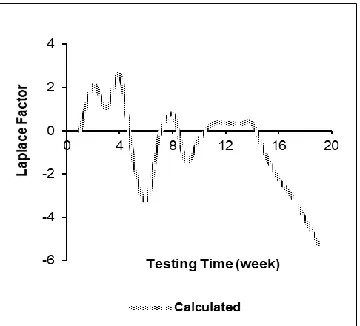
The software reliability data had been collected during 19 weeks of testing and debugging of PL/I application program test data of size 1,317,000 lines of code (LOC). Over the course of 19 weeks, 47.65 CPU hours were consumed, and 328 software faults were reported [34]. In this project, we assume that this dataset was observed from the testing phase after confirmation of the integration of all software components. Figure 6 traces the Laplace trend test. The values of the trend test that are oscillating between 2 and +2 indicate stable reliability till the 17th _{week. Except for the 5}th

week, we see decay, and because the decay does not last for long period, we should not pay attention to it. Stable reliability trend indicates that the corrective actions have no visible effect on reliability. In such situation the testing and debugging team must introduce new test sets. However, after 16th _{week, the}

behaviour becomes stable, which means that reliability grew monotonically. In such situation the system is used less or the reason behind this may also be due to unrecorded faults. Therefore, the testing and debugging team must take particular care [4], [6], and [33].

Fig. 6. Laplace test data trend

The resultant parameter estimation and the goodness-of-fit metrics in terms of SSE, Bias, Variation, and RMSPE of the models under comparison are tabulated in Table 2. According Table 2 we can see that the logistic function has lower metric values among the testing-effort functions under comparison. Therefore, the comparison criteria favour the logistic testing-effort function and, hence, adopted for further evaluation. It is worth mentioning that the exponential function fails to give any plausible estimation results.

Table 2. Parameter estimation & comparison criteria metrics results.

Functions Under Comparison

Parameter

Estimation Comparison Criteria

𝜸 𝒄 𝒓 SSE Bias Variation RMSPE Exponential * *

— — 1.12

* * * * Rayleigh 49.32 0.01₄ 99.5₀ 0.560 2.28 2.347

Weibull 799.2₂ 0.00₂ 297.₄ 3.362 4.12 3.987 Logistic 54.84 0.22₆ 13.0₃ 30.9₅ -0.062 1.31 1.311

* the function fails to give any plausible result.

— the component is not part of the corresponding function

The fitting of the testing-effort functions under comparison to the actual non-cumulative and cumulative testing-effort are graphically illustrated in Figures 7 and 8 respectively. From both Figures, we can observe that the logistic testing-effort function provides a better fit than the other functions under comparison. Therefore, the logistic testing-effort function provides more accurate description of resource consumption than other functions.

Fig. 7. Non-cumulative testing-effort curves

Fig. 8. Cumulative testing-effort curves

2182 perfect debugging or debugging efficiency ‗p‘ of the faults

encountered in the re-used components is lower than that encountered in the newly developed components and the error introduction or generated rate ‗α‘, reveals that the debugging process doesn‘t introduce any error for re-used components but it is not the case for newly-developed components.

Table 3. Parameter estimation.

Models Under Comparison

Parameter Estimation

𝒂 𝒃 , 𝒑 , 𝜶 , 𝒃 , 𝒑 , 𝜶 ,

Yamada et al. [14] 378.1₂ 0.470 — — 0.1 80 — — Shatnawi [15] 419.4₅ 0.532 — — 0.184 — — Proposed 300.6₄ 0.383 0.50₁ 0 0.771 0.98₈ 0.35

It is estimated that a total of 408.81 faults were detected in the 19 weeks including 108.17 faults were introduced or

generated, and out of them, only 336 were perfectly debugged and corrected as shown in Table 4.

Table 4. Results.

Initial Fault-Content

Effort Consumed

Total Fault-Content

Number of Fault-Introduced

Number of Fault-Corrected

𝒂 𝑾 𝒂 = 𝒂 + 𝜶 ∙ 𝒂 − 𝒂

300.64 46.55 408.81 108.17 335.53

The resultant goodness-of-fit metrics in terms of SSE, bias, variation and RMSPE of the proposed model compared with other existing models are given in Table 5. As given in Table 5, the overall values of SSE, bias, variance and RMSPE for the proposed model are the lowest. As results of comparison, we may conclude that the proposed modelling approach fits better than the other models under comparison for this actual software reliability data.

Table 5. Comparison criteria metrics results.

Models Under Comparison

Comparison Criteria SSE Bias Variation RMSPE Yamada et al. [14] 2374.7₃ -0.231 11.484 11.486

Shatnawi [15] 1757.6₆ -0.536 9.866 9.881 Proposed 1484.3₀ -0.180 9.079 9.081

As the software system composed of four components, two of them are re-used and the other two are newly-developed. Tables 6 and 7, reveal very important results that can be of immense help to the software developer and decision maker such as the initial fault-content, amount of testing-effort expenditure, total number of fault-content included the number of fault-introduced due to imperfect-debugging environment, and number fault-corrected for each of these components.

Table 6. Comparison criteria metrics results.

Models Under Comparison

Re-used Components Component 1 Component 2

𝒂 𝑾 𝒂 𝒂 𝑾 𝒂

Yamada et al. [14] 18.9 — — 18.9 18.9 — — 18.9 Shatnawi [15] 51.6 8.8 — 50.7 32.3 0.47 — 19.4 Proposed 45.1 8.8 45.1 24.3 15.0 0.47 15.0 2.2

— the component is not part of the corresponding model

Table 7. Comparison criteria metrics results.

Models Under Comparison

Newly Components

Component 3 Component 4

𝒂 𝑾 𝒂 𝒂 𝑾 𝒂

Yamada et al. [14] 170.₂ — — 145.₂ 170.₂ — — 145.₂ Shatnawi [15] 158.₁ 18.2 — 150.₁ 177.₄ 19.1 — 111.₆ Proposed 105.₂ 18.2 195.₇ 50.4 135.₃ 19.1 152.₉ 258.₆

— the component is not part of the corresponding model

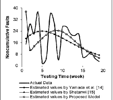
The fitting of the proposed model to the actual non-cumulative and cumulative software reliability data are graphically illustrated in Figure 9 and 10 respectively. From both Figures, we can observe that the proposed model is very close to the actual software reliability data and fits the data excellently well.

Fig. 9. Non-cumulative reliability curve

Fig. 10. Cumulative reliability growth curve

6 C

ONCLUSION

2183 component-based modelling in software reliability engineering,

that could be of immense help to the software project manager in monitoring and controlling the testing process closely and effectively allocating the resources in order to reduce the testing cost and to meet the given reliability requirements. Finally, this study provides a new insight into the development of software reliability modelling in distributed development environment. It has also demonstrated the integration of a set of existing non-homogenous Poisson process-based software reliability model. The resultant integrated component-based modelling approach has been validated and compared with other existing non-homogenous Poisson process based software reliability models by applying them on three software reliability data. The results were very promising. Today is a period of transition for neural network technology. As neural network can be described in a mathematical form and they have a significant advantage over analytical models, because they require only software reliability data history as input and no assumptions. The extension of our integrated component-based modelling approach to demonstrate the applicability of the neural network approach to the modelling of software reliability in distributed development environment, is an ongoing challenge that stimulates more future research efforts.

A

CKNOWLEDGMENT

The first author would like to emphases that much of the research that has found its way into this manuscript was carried out during her Thesis-based M.Sc. in Computer Science programme and she would also like to gratefully acknowledge the support of Al al-Bayt University.

R

EFERENCES

[1] Lavinia, C. Dobre, F. Pop, and V. Cristea,―A Failure Detection System for Large Scale Distributed Systems,‖ International Journal of Distributed Sys-tems and Technologies, vol. 2, no. 3, pp. 64–87, 2011. [2] J.D. Musa, Software Reliability Engineering: More Reliable Faster and Cheaper. 2nd edition, McGraw-Hill, 2004.

[3] M.R. Lyu, ―Software Reliability Engineering: A Roadmap,‖ Proc. Future of Software Engineering (FOSE‘07), IEEE Computer Society, Washington, DC, USA, pp. 153–170, 2007.

[4] O. Shatnawi, ―Measuring Commercial Software Operational Reliability: An Interdisciplinary Modelling Approach,― Eksploatacja i Niezawodność - Maintenance and Reliability, vol. 16, no. 4, pp.585– 594, 2014.

[5] P.K. Kapur, H. Pham, A. Gupta, and P.C. Jha, Software Reliability Assessment with OR Applications, Springer-Verlag, 2011.

[6] O. Shatnawi, ―An Integrated Framework for Developing Discrete-Time Modelling in Software Reliability Engineering,‖ Quality and Reliability Engineering International, vol. 32, no. 8, pp. 2925-2943, 2016.

[7] S. Yamada, Software Reliability Modeling: Fundamentals and Applications. Springer, 2014. [8] O. Shatnawi, ―Discrete Time NHPP Models for

Software Reliability Growth Phenomenon,‖ International Arab Journal of Information Technology, vol. 6, no. 2, pp. 124-131, 2009.

[9] IEEE Computer Society, ―IEEE Standard Glossary of

Software Engineering Terminology,‖ IEEE Standard 610.12-1990.

[10] Boehm and V.R. Basili, ―Software Defect Reduction Top 10 List,‖ Computer, vol. 34, no. 1, pp. 135–137, 2001.

[11] G. Tassey, ―The Economic Impacts of Inadequate Infrastructure for Software Testing,‖ Technical Report RTI Project Number 7007.011, National Institute of Standards and Technology, Gaithersburg, MD, USA, 2002.

[12] Jones, Applied software measurement: Global Analysis of Productivity and Quality. McGraw-Hill, 3rd edition, 2008.

[13] Y. Tamura, S. Yamada, and M. Mitsuhiro. ―A reliability assessment tool for distributed software development environment based on Java and J/Link,‖ European Journal of Operational Research, vol. 175, no. 1, pp. 435-445, 2006.

[14] S. Yamada, Y. Tamura, and M. Kimura, ―A Software Reliability Growth Model for A Distributed Development Environment,‖ Electronics and Communications in Japan - Part 3, vol. 83, no. 12, pp. 1–8, 2000.

[15] O. Shatnawi, ―Testing-effort dependent software reliability model for distributed systems‖, International Journal of Distributed Systems and Technologies, vol. 4, no.2, pp. 1-14, 2013.

[16] P.K. Kapur and A.K Bardhan, ―Testing effort control through software reliability modelling,‖ International Journal of Modelling and Simulation, vol. 22, no. 1, pp. 90–96, 2002

[17] P.K. Kapur, A. Gupta, O. Shatnawi, V.S.S. Yadavalli, ―Testing effort control using flexible software reliability growth model with change point,‖ International Journal of Performability Engineering, vol. 2, no. 3, pp.245-262, 2006.

[18] C.Y. Huang, S.Y. Kuo, and M.R. Lyu, ―An Assessment of Testing-Effort Dependent Software Reliability Growth Models,‖ IEEE Transactions on Reliability, vol. 56, no. 2, pp. 198-211, 2007.

[19] P.K. Kapur, O. Shatnawi, A.G. Aggarwal, and R. Kummar, ―Unified Framework for Developing Testing Effort Dependent Software Reliability Growth Models,‖ WSEAS Transactions on Systems, vol. 8, no. 4, pp. 521-531, 2009.

[20] S.Y. Kuo, C.Y. Huan, and M.R. Lyu, ―Framework for modelling software reliability using various testing-effort and fault-detection rates,‖ IEEE Transactions on Reliability, vol. 50, pp. 310-320, 2011.

[21] R. Peng, Y.F. Li, W.J. Zhang, and Q.P. Hu, ―Testing Effort Dependent Software Reliability Model for Imperfect Debugging Process considering both Detection and Correction, ―Reliability Engineering and System Safety, vol. 126, pp. 37–43, 2014.

[22] M.R. Lyu, Handbook of Software Reliability Engineering. McGraw-Hill, 1996.

[23] P.K. Kapur, A.K. Bardhan, and O. Shatnawi, ―Why Software Reliability Growth Modelling should Define Errors of Different Severity,‖ Quality Control and Applied Statistics, vol. 49, no. 6, pp. 699-702, 2004. [24] O. Shatnawi, ―Discrete time modelling in software

2184 391-398, 2009.

[25] S. Inoue and S. Yamada, ―Discrete Software Reliability Assessment with Discretized NHPP Models,‖ Computers and Mathematics with Applications, vol. 51, no. 2, pp. 161–170, 2006. [26] A.L. Goel and K. Okumoto, ―Time Dependent Error

Detection Rate Model for Software Reliability and other Performance Measures,‖ IEEE Transactions on Reliability, vol. 28, no. 3, pp. 206-211, 1979.

[27] S. Yamada, M. Ohba, and S. Osaki, ―S-shaped Reliability Growth Modelling for Software Error Detection,‖ IEEE Transactions on Reliability, vol. 32, pp. 475-478, 1983.

[28] W.C. Lim, ―Effects of reuse on quality, productivity and economics,‖ IEEE Transactions on Software, 11(5), pp. 23–30, 1994.

[29] J.D. Musa, A. Iannino, A. and K. Okumoto, Software Reliability: Measurement, Prediction, Applications. McGraw-Hill, 1987.

[30] H. Ohtera and S. Yamada, ―Optimal allocation and control problems for software-testing resource,‖ IEEE Transactions on Reliability, vol. 39, no. 2, pp. 171– 176, 1990.

[31] Z. Wang, K. Tang, and X. Yao, ―Multi-objective approaches to optimal testing resource allocation in modular software systems,‖ IEEE Transactions on Reliability, vol. 59, no. 3, pp. 563–575, 2010.

[32] C-T. Lin, ―Analyzing the Effect of Imperfect Debugging on Software Fault Detection and Correction Processes via a Simulation Framework, Mathematical and Computer Modelling, vol. 54, pp. 3046–3064, 2011.

[33] K. Kanoun, M. Kaaniche, and J-C. Laprie, ―Qualitative and Quantitative Reliability Assessment,‖ IEEE Software, vol. 14, pp. 77-87, 1997.