Reverse Sparse Representation for Single Image
Super-Resolution
Jian Xu
1,2,3*, Chunyu Wang
1,2,3, Jiulun Fan
1,2,31 Key Laboratory of Electronic Information Application Technology for Scene Investigation, Ministry of Public Security, Xi'an, 710121, China.
2 International Joint Research Center for Wireless Communication and Information Processing, Shaanxi, Xi'an, 710121, China.
3 Xi’an University of Posts and
Telecommunications, Xi’an 710121, China.
* Corresponding author. Tel.: (+86)17792510697; email: [email protected] Manuscript submitted June 11, 2018; accepted July 17, 2018.
doi: 10.17706/jcp.13.11 1246-1264.
Abstract: The key issue facing the machine learning based super-resolution (SR) method is how to describe the relationship between the low-resolution (LR) and high-resolution (HR) images. Sparse representation techniques have provided effective tools for this task. In classical coupled dictionary models, the most important issue is how to train two dictionaries to convert the HR and LR data samples to a unified feature subspace. To address this problem, this paper presents novel coupled dictionary training approach for SR. In the proposed model, reverse sparse representation constrains are employed to train coupled dictionaries to reduce the weaknesses of the SR problem. To avoid the alternative iteration and reduce the time complexity, the HR and LR dictionaries are trained in two steps. First, the HR dictionary is trained with the traditional single dictionary training algorithm. Next, according to the HR dictionary and the HR data set, the reverse sparse representations are prepared to generate the LR atoms. Finally, the LR dictionary is generated with reverse sparse representations and the LR data set. Experimental results demonstrate that our approach outperforms 7 related approaches.
Keywords: Super-resolution, sparse representation, dictionary training, non local mean regularization.
1.
Introduction
Super-resolution is a technology that magnifies low-resolution (LR) images into high-resolution (HR) image and simultaneously recovers the high frequency details [1]-[3]. Sparse representation is a popular tool for many real applications, especially in the image processing area [4]-[6]. In Super-resolution (SR), sparse representation is used as a tool to describe the relationship between the HR and the LR images [7], [8].
In the sparse representation model, the most important task is to design the dictionary. There are two methods to accomplish this task: one is to use a pre-specified linear transformation [9]-[11], and the other is to train a dictionary to fit a group of data samples [12]-[14].
Popular linear transformations, such as the Fourier or wavelet transformation[15], cannot always obtain the sparse coefficients for natural images. Therefore, the second strategy is considered a good
way to design dictionaries[16]. Engan et al. [17] presented the Method of Optimal Directions (MOD). This method updates the dictionary according to the fixed sparse coefficients and updates the sparse coefficient according to the fixed dictionary alternately by using the best solution. The Maximum A-posteriori Probability (MAP) [18] method employs the steepest descending direction to alternately update the sparse representation and the dictionary. The above two algorithms do not always converge. Aharon et al. [19] proposed the singular value decomposition (SVD) algorithm. The K-SVD algorithm updates the dictionary and sparse representation coefficient simultaneously with the singular vectors. This property improves the convergence rate. Mairal et al. [20] proposed various dictionary training algorithm to fit different tasks. Rubinstein et al. [21] proposed a double sparsity sparse representation method to combine the pre-specified linear transformation and the trained dictionary. This method can accelerate the dictionary training process. Several online dictionary training algorithms were proposed to reduce the memory requirement [20], [22].
The SR method based on sparse representation needs to train coupled dictionaries [23]. One dictionary corresponds to the LR image and the other corresponds to the HR image. Since the single dictionary training area has provided many experiences for this task, many researchers propose methods to transform the coupled dictionary training algorithm into the single dictionary training algorithm [13], [24]-[27]. Yang et al. [25] proposed a joint learning algorithm, which join the corresponding LR and HR data samples into a single data sample and subsequently uses a single dictionary training algorithm. The method proposed by Zeyde et al. [28] first trains the LR dictionary with a single dictionary training algorithm and later generates the HR dictionary with least-squares method. Xu et al. [29] proposed a coupled K-SVD algorithm to alternately update the corresponding HR and LR dictionary atoms. Wang [30] proposed a semi-coupled dictionary learning algorithm, which trains the LR and HR dictionaries and later trains another matrix to transform the LR sparse representation into an HR sparse representation.
In this work, we also focus on the coupled dictionary training task for SR based on sparse representation. To improve the reconstruction ability of the coupled dictionaries, we add two reverse sparse representation constraints on Yang's sparse representation model [25]. These constraints enforce the requirement that the corresponding dictionary atoms represent the corresponding components of the HR and LR patches. The algorithm trains the HR and LR dictionaries in two steps, which avoids alternate optimization among many variables. The reverse sparse representations bridge the HR and LR dictionaries, which reduces the weaknesses of the SR problem. Experimental results demonstrate the effectiveness and efficiency of the algorithm.
The remainder of this paper is organized as follows. Section 2 presents the proposed RSR algorithm. Section 3 provides the experimental results. Next, the Section 4 presents the study’s conclusions.
2.
Reverse Sparse Representation Algorithm
2.1.
SR Model Based on Sparse Representation
Single image SR aims to reconstruct an HR image as close as possible to the original HR image. Since the local patches redundantly repeat themselves in natural images, the sparse representation model operates on the local patches.
The sparse representation model is based on the following assumptions:
(1) The LR patches
X
{ }
x
i iN1 and HR patchesY
{ }
y
i Ni 1 can be sparse represented by twodictionaries x
m nlR
D
andD
y
R
mhn, whereN
is the number of patches, n is the number of thedictionary atoms, and l
(2) The corresponding LR and HR patches
( ,
x y
i i)
have similar sparse representations. The traditional coupled dictionary training model [26] is
i
2 2
2 2 1
, ,{ } 1
2 2
min
1, 1, 1, 2,
. . ,
x y N x yi i i i i
i
x y
r r
s t r n
D D α x D α y D α α
d d
‖ ‖ ‖ ‖ ‖ ‖
‖ ‖ ‖ ‖
(1)
where
α
i is the sparse representation for thei
th HR and LR training samples, x rd
andd
ry are ther
th dictionary atoms in the HR and LR dictionaries, respectively .The sparse representation model assumes that a natural signal is composed of a small group of dictionary atoms [31].
The traditional model considers the sparse representations of data samples, but does not consider the structure of the dictionary atoms. Therefore, we propose a coupled dictionary training model as follows:
2 2 2 2
2 2 2 2
, , ,
min
x y
x y x y
D D A B X D A Y D A D XB D YB
‖ ‖ ‖ ‖ ‖ ‖ ‖ ‖ (2)
2 2 0 1 0 2
. . 1, 1, ,
1, 2, , 1, 2, ,
x y
r r i r
s t T T
r n i N
d d α β
‖ ‖ ‖ ‖ ‖ ‖ ‖ ‖
where A
α α1, 2, ,αN
andB
β β
1,
2,
,
β
n
are the sparse representation matrixes.T
1 andT
2 arethe sparseness constraints.
β
r is the sparse representation corresponding to x rd
andd
ry with respectto
X
and Y .The model (2) adds two reverse representation constraint items and one sparse constraint item to the model (1).
The motivation to add these constraints is stated below.
The corresponding HR and LR dictionary atoms should represent the HR and LR version of the same image component. To make the representations sufficiently sparse, one atom only supports a small space area such that it better approximates the data groups. Therefore, a given atom can be considered as a cluster center for a given cluster group. The cluster center only better approximates a small number of data samples. When using the whole data set to form a dictionary, every atom can be well represented by a small number of data samples.
There are four variables in the above model: the LR dictionary x
D
, the HR dictionaryD
y and the spare representation matrixesA
α α
1,
2,
,
α
N
and B
β β1, 2, ,βn
. The most important issue is how to optimum these variables.2.2.
Details of the Proposed Algorithm
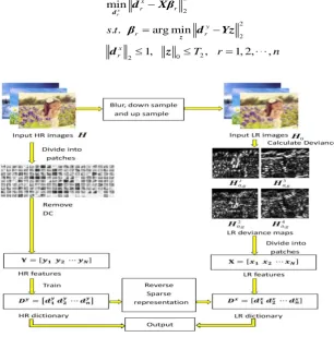
Fig. 1 illustrates the framework of the proposed algorithm.
First, we prepare proper training sets. The HR training image
H
is selected from the natural images.H
is down sampled with a bicubic interpolation to generate the LR training imageL
. Since the bicubic interpolation can recover reliable low frequency and middle frequency information, we up sampled the LR training image into the desired size with bicubic interpolation and we denote the up sampled image asH
0. We use the first and second order deviances as the features of the LRpatches[32]. We use four filters
f
1
[ 1, 0,1]
,f
2
f
1T,3
[1, 0, 2, 0,1]
f
,f
3
f
4Tto calculate thedeviance maps of
H
0 and denoted them as 1 2 3 4 0,g, 0,g, 0,g, 0,gH H H H . The LR training set
{ }
=1 N i iX
x
isFig. 1. The flowchart of the proposed algorithm.
In model (4), the HR dictionary atom y r
d
is reversely represented by HR training samplesY
. Next, the reverse sparse representationβ
r(1
r
n
)
is used to calculate the LR dictionary atoms.Therefore, the model (4) can be separated into two optimization problems
2
2 0 2
arg min
y,
,
1, 2,
,
r
z r
T r
n
β
d
Yz
z
(5)2
2
2
min
. . 1, 1, 2, ,
x r x r r x r
s t r n
d d Xβ d (6) coordinate into a vector. The HR training set
Y
{ }
y
i iN=1 is obtained by dividingH
into patches and subtracting their mean values. The patch size is denoted asq q
, the dimension ofx
iis denoted asl
m
and the dimension ofy
i is denoted as hm
,m
l
4
q
2 and h 2m
q
.To obtain an accurate HR dictionary y
D
, we solve the standard sparse coding dictionary training problem 2 2 , 1 1 0 2 min. . 1, , 1, 2, ,
y i N y i i i y rs t T r n
D α
i
y D α
d α
(3)
The next issue is how to estimate the LR dictionary x
D
that can provide a similar sparserepresentation
α
i for the LR training samplex
i. We use model (4) to calculate the LR dictionary. 2 2 2 2 2 0 2 min. . arg min
1, , 1, 2, ,
x r x r r y r r x r s t
T r n
d z d Xβ
β d Yz
d z
(4)
Task:
Estimate the best possible coupled dictionaries x
D
and yD
to represent the LR training samples
N1 i ix
and HR training samples
1 N i i
y
by solving model (2).Doing the following steps:
1: Train the HR dictionary
D
y by solving model (3) with K-SVD dictionary training algorithm [19, 34];2: Calculate
β
r according to formula (5) by OMP algorithm[35];3: Obtain the LR dictionary by optimum model (6)
Therefore, the HR image Y and the LR image
X
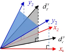
have the similar sparse representation matrix. If we neglect the filtering effect of the HR image, the LR patch can be considered as the down sampled version of the HR patch, as shown in Fig. 2. Suppose we have a proper HR dictionary yD
via the traditional single dictionary training algorithm. The next task is to calculate a reliable LR dictionaryx
D
according toD
y. We consider the given LR patch as the projection of the corresponding HR patch in the low dimensional space. Supposex
1 andx
2 are the projections ofy
1 andy
2 in the lowdimensional space and HR atom y r
d
is spanned byy
1 andy
2, the LR atom x rd
is obviously spannedby
x
1 andx
2. For the SR problem, it is an under-determined problem to calculate HR features according to LR features, but reversely it is an over-determined problem to calculate LR features according to HR features. Therefore, it is more reliable to calculate the LR information according to the HR information. The alternate optimization among many variables is avoided. Therefore, the computational complexity is also reduced.Fig. 2. Explanation of the proposed algorithm.
2.3. Analysis of the Proposed Algorithm
Suppose
α
ˆ
i is the estimated value ofα
i, andβ
ˆ
r is the estimated value ofβ
r. It is easy to find thatˆ
y
Y
D A
,D
y
YB
ˆ
andD
x
XB
ˆ
according to formula (3)-(4), whereA
ˆ
α α
ˆ ˆ
1,
2,
,
α
ˆ
N
and1 2 n
ˆ ˆ
ˆ
ˆ
,
,
,
B
β β
β
.The traditional warp-blur model [33]supposes the LR image
X
is related to the HR image Y by
X
SEY
, whereE
describes such phenomena as the blur degradation by optical blur, motion blur, and sensor point spread function (PSF).S
is the down sampling matrix. The observation noise isneglected.
ˆ
ˆ
ˆ
ˆ
ˆ
ˆ
y x
X
SEY
SED A
SEYBA
XBA
D A
3.
Experiments
In this section, we will first introduce the experimental settings, and compare our algorithm with 7 state-of-the-art algorithms. Next, we will discuss two influential factors for the proposed algorithm, i.e., the patch size and the dictionary size. We also discuss the effect of the post-processing procedures. Finally, we will show the time complexity of the proposed algorithm.
3.1.
Experimental Setting
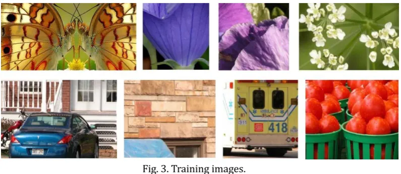
In our experiments, we magnify the input LR image both by the factors of 3 and 4. We collected 100,000 coupled patches as the external training database from the software package about the literature[25]. Fig. 3 shows several training images. The color training images are transformed into gray images. We only use the patches which contain the texture information and the smooth patches are discarded.
Fig. 3. Training images.
Fig. 4 shows some LR test images. The test images are transformed from RGB color space to YCbCr color space. Y is the luminance component, and Cb and Cr are the chrominance components. Since the human visual system is more sensitive to the luminance component than the chrominance components[36], we only reconstruct the luminance component with the proposed algorithm. The chrominance components are reconstructed by bicubic interpolation. To further enhance the quality of the SR results, the non-local means (NLM) regularization [37] is applied to the output of the abovementioned approach.
3.2.
Comparison with Other Methods
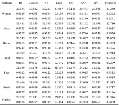
Table 1. PSNRs, SSIMs and FSIMs for the Reconstructed Images by Different Methods (3x). In Each Table Cell, the First Line is PSNR Value, the Second Line is SSIM Value, and the Third Line is FSIM Value
Methods BI Glasner NE Yang SAI ANR IPR Proposed
Woman
29.384 30.562 30.261 31.087 30.141 30.471 29.805 31.260
0.8949 0.9095 0.8984 0.9199 0.9043 0.9131 0.8997 0.9262
0.8993 0.9206 0.9105 0.9285 0.9151 0.9189 0.9055 0.9291
Lena
31.411 32.155 32.195 32.595 32.082 32.102 31.698 32.710
0.8252 0.8433 0.8402 0.8509 0.8409 0.8497 0.8837 0.8612
0.9707 0.9835 0.9832 0.9844 0.9826 0.9746 0.9750 0.9850
Horse
33.543 33.783 34.123 34.967 34.291 34.027 33.798 35.053
0.9065 0.9111 0.9116 0.9249 0.9162 0.9228 0.9106 0.9329
0.9247 0.9326 0.9340 0.9440 0.9373 0.9380 0.9300 0.9476
Child
32.899 33.261 33.125 33.611 33.336 32.631 33.065 33.913
0.8001 0.8169 0.8133 0.8242 0.8183 0.8452 0.8090 0.8362
0.8881 0.9113 0.9077 0.9145 0.9138 0.9089 0.8986 0.9209
Face
33.939 34.578 34.322 35.139 34.674 34.313 34.052 35.536
0.9042 0.9165 0.9122 0.9225 0.9169 0.9015 0.9104 0.9332
0.9808 0.9899 0.9891 0.9914 0.9893 0.9817 0.9850 0.9915
Koala
30.466 31.160 31.081 31.530 30.994 31.030 30.781 31.913
0.8186 0.8450 0.8400 0.8551 0.8416 0.8431 0.8338 0.8717
0.8797 0.9055 0.9019 0.9123 0.9048 0.9037 0.8338 0.9196
Starfish 28.102 28.691 28.678 29.055 28.733 28.423 28.369 31.346
0.8126 0.8359 0.8319 0.8464 0.8365 0.8383 0.8263 0.9050
We compare our algorithm with 7 existing algorithms, including: Bicubic Interpolation(BI) [38], Neighbor Embedding (NE)[39], Glasner's method[40], Soft-decision adaptive interpolation (SAI)[41], Yang's method [25], Anchored Neighborhood Regression (ANR) [42] and In Place Regression (IPR) [43]. To make a fair comparison, we use the same training set for all these methods. We compare the peak signal-to-noise ratio (PSNR), structural similarity (SSIM)[44], and feature similarity (FSIM)[45] of the reconstructed HR images in Table 1 and Table 2. PSNR, SSIM and FSIM are all quantitative evaluations of the images. When the peak intensity value of the image is determined to be 255, the PSNR is only related to the squared intensity differences of the reconstructed and the original HR images. Many references have demonstrated that it is not very well matched to perceived visual quality [44]. Therefore, the SSIM and the FSIM are proposed to solve the problem. SSIM evaluates the perceived change in structural information, and the FSIM evaluates the consistency of the features extracted by the Fourier waves. Table 1 and Table 2 show that the RSR method performs better than the other methods.
0.8828 0.8999 0.8949 0.9071 0.9008 0.8988 0.8915 0.9396
Flower
30.144 30.669 30.613 30.992 30.602 30.410 30.304 29.543
0.8710 0.8853 0.8774 0.8938 0.8827 0.8842 0.8776 0.8653
0.9140 0.9281 0.9217 0.9331 0.9282 0.9247 0.9196 0.9168
Castle
26.211 26.534 26.554 26.710 26.442 26.948 26.349 27.202
0.7984 0.8145 0.8127 0.8215 0.8113 0.8288 0.8076 0.8428
0.8513 0.8676 0.8650 0.8702 0.8644 0.8727 0.8578 0.8877
Lama
36.015 36.901 36.723 37.712 36.789 37.365 36.423 37.666
0.9457 0.9516 0.9473 0.9585 0.9515 0.9577 0.9490 0.9633
0.9464 0.9549 0.9511 0.9613 0.9544 0.9590 0.9508 0.9648
Avg.
31.211 31.829 31.768 32.340 31.808 31.732 31.464 32.434
0.8577 0.8730 0.8685 0.8818 0.8720 0.8818 0.8708 0.8898
0.9138 0.9294 0.9259 0.9348 0.9291 0.9281 0.9207 0.9380
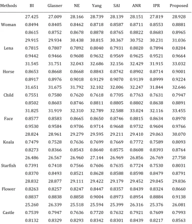
Table 2. PSNRs, SSIMs and FSIMs for the Reconstructed Images by Different Methods (4x). In Each Table Cell, the First Line is PSNR Value, the Second Line is SSIM Value, and the Third Line is FSIM Value
Methods BI Glasner NE Yang SAI ANR IPR Proposed
Woman
27.425 27.009 28.166 28.739 28.139 28.151 27.819 28.928
0.8494 0.8405 0.8462 0.8718 0.8587 0.8711 0.8553 0.8881
0.8615 0.8752 0.8678 0.8878 0.8765 0.8822 0.8683 0.8965
Lena
29.915 29.934 30.438 30.815 30.367 30.752 30.231 31.036
0.7815 0.7807 0.7892 0.8040 0.7931 0.8020 0.7894 0.8204
0.9442 0.9466 0.9608 0.9632 0.9569 0.9625 0.9521 0.9664
Horse
31.545 31.751 32.043 32.686 32.156 32.429 31.915 33.032
0.8653 0.8668 0.8668 0.8843 0.8742 0.8902 0.8714 0.9001
0.8917 0.8976 0.9018 0.9129 0.9070 0.9139 0.8999 0.9224
Child
31.651 31.675 31.792 32.102 32.006 32.247 31.844 32.646
0.7551 0.7580 0.7620 0.7618 0.7705 0.7763 0.7631 0.7947
0.8502 0.8603 0.8746 0.8811 0.8805 0.8802 0.8638 0.8891
Face
31.825 31.919 32.310 32.789 32.588 33.024 32.116 33.455
0.8577 0.8583 0.8665 0.8650 0.8746 0.8815 0.8634 0.8978
0.9530 0.9584 0.9706 0.9714 0.9668 0.9732 0.9604 0.9766
Koala
28.824 28.961 29.279 29.595 29.211 29.410 29.063 30.070
0.7479 0.7528 0.7636 0.7699 0.7669 0.7772 0.7589 0.8093
0.8273 0.8366 0.8543 0.8640 0.8575 0.8608 0.8393 0.8764
Starfish
26.486 26.567 26.960 27.144 26.969 26.856 26.769 27.758
0.7391 0.7418 0.7566 0.7606 0.7635 0.7724 0.7530 0.8031
0.8370 0.8493 0.8521 0.8628 0.8588 0.8598 0.8479 0.8791
Flower
28.832 28.877 29.111 29.422 29.179 29.452 29.045 29.836
0.8263 0.8257 0.8247 0.8447 0.8357 0.8439 0.8324 0.8660
0.8837 0.8838 0.8858 0.9004 0.8973 0.8954 0.8884 0.9138
Castle
25.260 26.339 25.518 25.594 25.399 26.316 25.376 26.081
0.7539 0.7947 0.7636 0.7720 0.7632 0.7921 0.7609 0.7993
Lama
33.948 34.088 34.429 35.057 34.574 33.996 34.187 35.527
0.9153 0.9149 0.9153 0.9284 0.9223 0.9270 0.9171 0.9406
0.9181 0.9211 0.9241 0.9355 0.9291 0.9308 0.9212 0.9442
Avg.
29.5711 29.712 30.005 30.394 30.059 30.263 29.837 30.837
0.8092 0.8134 0.8155 0.8263 0.8223 0.8334 0.8165 0.8519
0.8780 0.8862 0.8921 0.9013 0.8961 0.9003 0.8863 0.9121
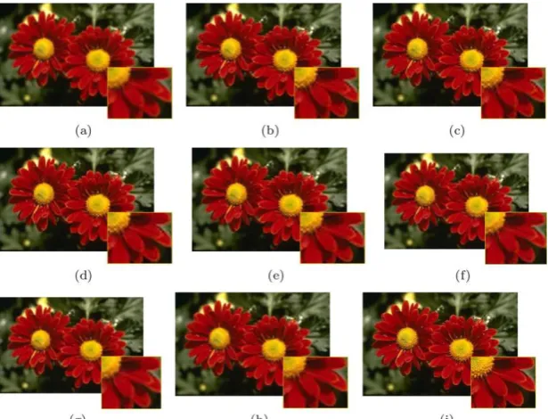
Fig. 5. Visual comparison of the “Flower” images (3x). (a)BI. (b) Glasner. (c) NE. (d)SAI. (e) Yang. (f) ANR. (g) IPR. (g) Proposed RSR. (i) Ground truth. (Refer to the electrical version and zoom in for better
comparison.).
Fig. 6. Visual comparison of the “Flower” images (4x). (a)BI. (b) Glasner. (c) NE. (d)SAI. (e) Yang. (f) ANR. (g) IPR. (g) Proposed RSR. (i) Ground truth. (Refer to the electrical version and zoom in for better
Fig. 7. Visual comparison of the “Horse” images (3x). (a)BI. (b) Glasner. (c) NE. (d)SAI. (e) Yang. (f) ANR. (g) IPR. (g) Proposed RSR. (i) Ground truth. (Refer to the electrical version and zoom in for better
comparison.).
Fig. 8. Visual comparison of the “Horse” images (4x). (a)BI. (b) Glasner. (c) NE. (d)SAI. (e) Yang. (f) ANR. (g) IPR. (g) Proposed RSR. (i) Ground truth. (Refer to the electrical version and zoom in for better
Fig. 9. Visual comparison of the “Castle” images (3x). (a)BI. (b) Glasner. (c) NE. (d)SAI. (e) Yang. (f) ANR. (g) IPR. (g) Proposed RSR. (i) Ground truth. (Refer to the electrical version and zoom in for better
comparison.).
Fig. 10. Visual comparison of the “Castle” images (4x). (a)BI. (b) Glasner. (c) NE. (d)SAI. (e) Yang. (f) ANR. (g) IPR. (g) Proposed RSR. (i) Ground truth. (Refer to the electrical version and zoom in for better
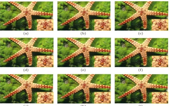
To substantiate the above assessment, it is observed that the pistil of the flower recovered by other methods lacks details. In contrast, RSR recovers the pistil more precisely than other methods. RSR also recovers correct spot shapes on the horseshoe and the window shapes on the castle without undesired artifacts. The textures on the starfish are clearer than those that results from other methods. It is clear that the SR results of RSR are more competitive than the other methods.
3.3.
Effects of the Patch Size and Overlap
Experimentally, we find that the SR results of RSR are highly correlated with the patch size. To obtain the optimal patch size, we trained 4 groups of dictionaries corresponding to different patch sizes:
3 3
,5 5
,7 7
and9 9
. We apply them to the same test images for comparison. The results are evaluated in PSNR and SSIM. To avoid the influence of the post-processing procedure, these results Fig. 11. Visual comparison of the “Starfish” images (3x). (a)BI. (b) Glasner. (c) NE. (d)SAI. (e) Yang. (f) ANR. (g) IPR. (g) Proposed RSR. (i) Ground truth. (Refer to the electrical version and zoom in for bettercomparison.).
Fig. 12. Visual comparison of the “Starfish” images (4x). (a)BI. (b) Glasner. (c) NE. (d)SAI. (e) Yang. (f) ANR. (g) IPR. (g) Proposed RSR. (i) Ground truth. (Refer to the electrical version and zoom in for better
are all outputs without NLM.
Fig. 13. Average PSNR and SSIM values for different patch sizes and overlaps. (a)PSNR values. (b)SSIM values. The blue bars correspond to the 3x magnification. The red bars correspond to the 4x
magnification.
Fig. 13 shows the average PSNR and SSIM values with different patch sizes and overlaps. We can see that the
5 5
with 3 pixels overlapped obtains the best PSNR and SSIM values both for the 3x and 4x magnifications.Fig. 14 shows the visual observations of different patch sizes. We can see that the smaller patch size recovers more details, but the number of artifacts also increase. Larger patch size introduces fewer artifacts, but the results are smoother.
Fig. 14. Visual comparison of “Woman” images with different patch sizes (4x). (a)3×3 with 1 pixel overlapped. (b)5×5 with 3 pixels overlapped. (c)7×7 with 5 pixels overlapped. (c)9×9 with 5 pixels
overlapped.
3.4. Effects of Dictionary Size
The dictionary size greatly affects the results and the time costs of the proposed algorithm. Since the dimension of LR feature is 100 for the patch size
5 5
, the size of the over complete dictionary should be more than 100 for reliable learning. For a fair comparison, these results are all outputs without NLM. The sparseness constraintsT
1 is set to ben
/ 4
andT
2 is set to beN
/ 30
. Table 4 and 5 show3.5.
Effectiveness of the Post-Processing Procedure
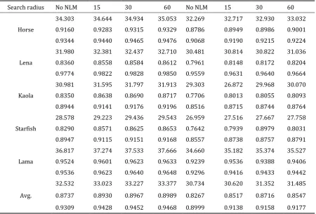
To further improve the quality of the output images, we employ several post-processing procedures. The non-local means (NLM) [37] regularization is based on the prior that the local image patches redundantly repeat themselves in different places in the same scale. The similar patches found from different locations are considered to be multiple observations of the target patch. The search radius greatly affects the result of the NLM. Table 6 shows the PSNR, SSIM and FSIM values of different searching radiuses. It is obvious that the post-processing procedure can suppress the artifacts and preserve the sharp edges. Fig. 15 compares the visual quality before and after the NLM enhancement. As shown, the NLM can effectively improve the quality of the output HR image. Since more reliable neighbors can be found in a larger area, the NLM obtains higher PSNR, SSIM and FSIM values with a larger search radius. However, a large search radius leads to high time costs. For a
321 481
dimensional image, the search radius of 15 pixels costs approximately 110s, the search radius of 30 pixels costs approximately 850s, and the search radius of 60 pixels costs approximately1.2 10
4s.Table 4. PSNRs, SSIMs and Time Costs Values with Different Dictionary Sizes (3x)
Dictionary Sizes 128 256 384 512
Woman 30.142 30.232 30.301 30.338
0.9051 0.9063 0.9076 0.9083
208.7 246.6 341.2 392.3
Flower 30.483 30.516 30.536 30.562
0.8798 0.8807 0.8814 0.8821
211.3 251.1 346.5 409.6
Lama 36.730 36.792 36.853 36.886
0.9517 0.9523 0.9527 0.9530
209.5 248.1 343.9 416.2
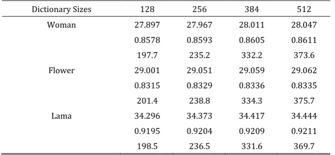
Table 5. PSNRs, SSIMs and Time Costs Values with Different Dictionary Sizes (4x)
Dictionary Sizes 128 256 384 512
Woman 27.897 27.967 28.011 28.047
0.8578 0.8593 0.8605 0.8611
197.7 235.2 332.2 373.6
Flower 29.001 29.051 29.059 29.062
0.8315 0.8329 0.8336 0.8335
201.4 238.8 334.3 375.7
Lama 34.296 34.373 34.417 34.444
0.9195 0.9204 0.9209 0.9211
198.5 236.5 331.6 369.7
/10
N
,N
/ 20
,N
/ 30
,N
/ 40
to choose the bestT
2. We find the best sparseness values areT
1
64
Fig. 15. Visual comparison of the “Flower” image by different search radius (4x) (a)Without NLM. (b)Search radius is 15. (c)Search radius is 30. (d)Search radius is 60.
Table 6. PSNRs, SSIMs and FSIMs for Different Search Radius in NLM
Search radius No NLM 15 30 60 No NLM 15 30 60
Horse
34.303 34.644 34.934 35.053 32.269 32.717 32.930 33.032
0.9160 0.9283 0.9315 0.9329 0.8786 0.8949 0.8986 0.9001
0.9344 0.9440 0.9465 0.9476 0.9068 0.9190 0.9215 0.9224
Lena
31.980 32.381 32.437 32.710 30.481 30.814 30.822 31.036
0.8360 0.8558 0.8584 0.8612 0.7961 0.8148 0.8172 0.8204
0.9774 0.9822 0.9828 0.9850 0.9559 0.9631 0.9640 0.9664
Kaola
30.981 31.595 31.797 31.913 29.303 26.872 29.968 30.070
0.8350 0.8638 0.8690 0.8717 0.7706 0.8013 0.8055 0.8093
0.8944 0.9141 0.9176 0.9196 0.8516 0.8715 0.8744 0.8764
Starfish
28.578 29.223 29.436 29.543 26.959 27.516 27.667 27.758
0.8290 0.8571 0.8625 0.8653 0.7642 0.7939 0.8979 0.8031
0.8947 0.9115 0.9151 0.9168 0.8557 0.8738 0.8757 0.8791
Lama
36.817 37.274 37.533 37.666 34.660 35.182 35.374 35.527
0.9524 0.9601 0.9623 0.9633 0.9239 0.9536 0.9388 0.9406
0.9536 0.9623 0.9640 0.9648 0.9296 0.9416 0.9433 0.9442
Avg.
32.532 33.023 33.227 33.377 30.734 30.620 31.352 31.485
0.8737 0.8930 0.8967 0.8989 0.8267 0.8517 0.8716 0.8547
0.9309 0.9428 0.9452 0.9468 0.8999 0.9138 0.9158 0.9177
3.6.
Time Consumption of Dictionary Training
According to the literature [19], the HR dictionary training procedure for the first step needs
1
O m NT nt
h flops, wheret
is the iteration number. The reverse sparse representations for eachatom can be found in
O m NT
h 2
flops. The procedure to generate the LR dictionary requires
1
O m T n
l flops. Therefore, the proposed dictionary training algorithm requires
1 2 1
learning algorithm [25], we do experiments on a PC running 8 cores of AMD FX-8150 CPU. The cores all iterate 10 times. The time costs of training dictionaries of different dictionary sizes n are
shown in Table 7, which demonstrates that the proposed dictionary training algorithm is more efficient than the joint learning algorithm.
Table 7. Comparison of Processing Time of Coupled Dictionary Training by Different Dictionary Size (s)
Dictionary Sizes 128 256 512
Yang 1915 2989 3686
Proposed 171 366 1010
4.
Conclusions
In this paper, we propose a coupled dictionary training method for a single image super-resolution. We train the HR dictionary first with traditional single dictionary training algorithm. Next, we generate the LR dictionary with a reverse dictionary training algorithm. Finally, an NLM based enhancement is applied to further improve the quality of the output HR image. The experimental results demonstrate that the proposed algorithm obtains a better reconstruction performance than 7 related works and has low time cost. However, there are still unrecovered details on the SR results. In our future research, we will attempt to find nonlinear relationships between the LR and HR features and try to recover more details by using nonlinear methods. The strategy of reverse sparse representation is a good choice to provide transformation tools for the machine learning communication known as "machine community" which focuses on describing two related situations (such as illumination change and contrast change).
Acknowledgement
This work was supported by the National Natural Science Foundation of China under Grant 61601362, Grant 41874173, Grant 61571361, Grant 61671377, Grant 41504115. New Star Team of Xi'an University of Posts and Telecommunications xyt2016-01.
References
[1] Xu, J., Chang, Z., & Fan, J. (2015). Image super-resolution by mid-frequency sparse representation and total variation regularization. Journal of Electronic Imaging, 24(1), 013039.
[2] Zhang, K., Tao, D., & Gao, X. (2017). Coarse-to-fine learning for single-image super-resolution. IEEE Transactions on Neural Networks and Learning Systems, 28(5), 1109-1122.
[3] Zeng, X., & Hou, S. (2017). Manifold-regularization super-resolution image reconstruction. Journal of Computers (Taiwan), 28(1), 119-136.
[4] Li, J., Gong, W., & Li, W. (2015). Dual-sparsity regularized sparse representation for single image super-resolution. Information Sciences, 298, 257-273.
[5] Dai, Q., Yoo, S., & Kappeler, A. (2017). Sparse representation-based multiple frame video super-resolution. IEEE Transactions on Image Processing, 26(2), 765-781.
[6] Hao, Y., Zhang, L., & Zhang, D. (2017). The fusion of gabor feature and sparse representation for face recognition. Journal of Computers (Taiwan), 28(2), 247-259.
[7] Deng, L., Guo, W., & Huang, T. (2016). Single image super-resolution by approximated heaviside functions. Information Sciences, 348, 107-123.
[9] Nazzal, M., & Ozkaramanli, H. (2014). Wavelet domain dictionary learning-based single image superresolution. Signal, Image and Video Processing, 1-11.
[10] Chavez-Roman, H., & Ponomaryov, V. (2014). Super resolution image generation using wavelet domain interpolation with edge extraction via a sparse representation. IEEE Geoscience and Remote Sensing Letters, 11(10), 1777-1781.
[11] Nazzal, M., & Ozkaramanli, H. (2012). Single image super resolution using sparsity and dictionary learning in wavelet domain. Proceedings of Signal Processing and Communications Applications Conference (pp. 1-4). Turkey: Mugla.
[12] Yu, J., Gao, X., & Tao, D. (2014). A unified learning framework for single image super-resolution. IEEE Transactions on Neural Networks and Learning Systems, 25(4), 780-792.
[13] Bao, C., Ji, H., & Quan, Y. (2016). Dictionary learning for sparse coding: Algorithms and convergence analysis. IEEE Transactions on Pattern Analysis and Machine Intelligence, 38(7), 1356-1369.
[14] Jing, X., Zhu, X., & Wu, F. (2017). Super-resolution person re-identification with semi-coupled low-rank discriminant dictionary learning. IEEE Transactions on Image Processing, 26(3), 1363-1378. [15] Kumar, N., & Sethi, A. (2018). Super resolution by comprehensively exploiting dependencies of
wavelet coefficients. IEEE Transactions on Multimedia, 20(2), 298-309.
[16] Ahmadi, K., & Salari, E. (2017). Single-image super resolution using evolutionary sparse coding technique. IET Image Processing, 11(1), 13-21.
[17] Engan, K., Aase, S. O., & Husoy, J. H. (2000). Multi-frame compression: Theory and design. Signal Processing, 80(10), 2121-2140.
[18] Lewicki, M. S., & Sejnowski, T. J. (2000). Learning overcomplete representations. Neural Computation, 12(2), 337-365.
[19] Aharon, M., Elad, M., & Bruckstein, A. (2006). K-SVD: An algorithm for designing overcomplete dictionaries for sparse representation. IEEE Transactions on Signal Processing, 54(11), 4311-4322. [20] Mairal, J., Bach, F., & Ponce, J. (2009). Online dictionary learning for sparse coding. Proceedings of
Annual International Conference on Machine Learning (pp.689-696). Canada: Montreal, QC.
[21] Rubinstein, R., Zibulevsky, M., & Elad, M. (2010). Double Sparsity: Learning Sparse Dictionaries for Sparse Signal Approximation, 58(3), 1553-1564.
[22] Szabo, Z., Poczos, B., & Lorincz, A. (2011). Online group-structured dictionary learning. Proceedings of IEEE Conference on Computer Vision and Pattern Recognition (pp. 2865-2872). USA: Colorado Springs.
[23] Dang, C., & Radha, H. (2017). Fast single-image super-resolution via tangent space learning of high-resolution-patch manifold. IEEE Transactions on Computational Imaging, 3(4), 605-616. [24] Yang, J., Wright, J., & Huang, T. (2008). Image super-resolution as sparse representation of raw
image patches. Proceedings of IEEE Conference on Computer Vision and Pattern Recognition (pp. 1-8). USA: Anchorage.
[25] Yang, J., Wright, J., & Huang, T. S. (2010). Image super-resolution via sparse representation. IEEE Transactions on Image Processing, 19(11), 2861-2873.
[26] Yang, J., Wang, Z., & Lin, Z. (2012). Coupled dictionary training for image super-resolution. IEEE Transactions on Image Processing, 21(8), 3467-3478.
[27] Tang, Y., & Shao, L. (2017). Pairwise operator learning for patch-based single-image super-resolution. IEEE Transactions on Image Processing, 26(2), 994-1003.
[28] Zeyde, R., Protter, M., & Elad, M. (2010). On single image scale-up using sparse-representation. Lecture Notes in Computer Science, 6920(1), 711-730.
Proceedings of IEEE International Conference on Image Processing (pp. 3910-3914). Paris, France. [30] Wang, S., Zhang, L., & Liang, Y. (2012). Semi-coupled dictionary learning with applications to image
super-resolution and photo-sketch synthesis. Proceedings of IEEE Conference on Computer Vision and Pattern Recognition (pp. 2216-2223). RI, USA: Providence.
[31] Baraniuk, R. G., Candes, E., & Elad, M. (2010). Applications of sparse representation and compressive sensing. Processings of the IEEE, 98(6), 906-909.
[32] Chen, H., He, X., & Qing, L. (2017). Single image super-resolution via adaptive transform-based nonlocal self-similarity modeling and learning-based gradient regularization. IEEE Transactions on Multimedia, 19(8), 1702-1717.
[33] Katsaggelos, A. K., Molina, R., & Mateos, J. (2007). Super Resolution of Images and Video (1st ed.). California, US: Morgan & Claypool Publishers.
[34] Smith, L. N., & Elad, M. (2013). Improving dictionary learning: Multiple dictionary updates and coefficient reuse. IEEE Signal Processing Letters, 20(1), 79-82.
[35] Rubinstein, R., Zibulevsky, M., & Elad, M. (2008). Efficient implementation of the K-SVD algorithm using batch orthogonal matching pursuit. CS Technion.
[36] Chen, X., & Qi, C. (2014). Nonlinear neighbor embedding for single image super-resolution via kernel mapping. Signal Processing, 94(1), 6-22.
[37] Zhang, K., Gao, X., & Tao, D. (2012). Single image super-resolution with non-local means and steering kernel regression. IEEE Transactions on Image Processing, 21(11), 4544-4556.
[38] Hou, H., & Andrews, H. (1978). Cubic splines for image interpolation and digital filtering. IEEE Transactions on Acoustics, Speech and Signal Processing, 26(6), 508-517.
[39] Chang, H., Yeung, D. Y., & Xiong, Y. (2004). Super-resolution through neighbor embedding. Proceedings of IEEE Computer Society Conference on Computer Vision and Pattern Recognition (pp. 275-282). Washington, DC, USA.
[40] Glasner, D., Bagon, S., & Irani, M. (2009). Super-resolution from a single image. Proceedings of IEEE International Conference on Computer Vision (pp. 349-356). Kyoto, Japan.
[41] Zhang, X., & Wu, X. (2008). Image interpolation by adaptive 2-D autoregressive modeling and soft-decision estimation. IEEE Transactions on Image Processing, 17(6), 887-896.
[42] Timofte, R., De Smet, V., & Van Gool, L. (2013). Anchored neighborhood regression for fast example-based super-resolution. IEEE International Conference on Computer Vision (pp. 1920-1927). Portland, Oregon, USA.
[43] Yang, J., Lin, Z., & Cohen, S. (2013). Fast image super-resolution based on in-place example regression. Proceedings of IEEE Conference on Computer Vision and Pattern Recognition (pp. 1059-1066). Portland, OR, USA.
[44] Wang, Z., Bovik, A. C., & Sheikh, H. R. (2004). Image quality assessment: From error visibility to structural similarity. IEEE Transactions on Image Processing, 13(4), 600-612.
[45] Zhang, L., Zhang, L., & Mou, X. (2011). FSIM: A feature similarity index for image quality assessment. IEEE Transactions on Image Processing, 20(8), 2378-2386.
has published the following articles, including:
[1] Xu, J., Chang, Z., & Fan, J. (2017). Super-resolution via adaptive combination of color channels. Multimedia Tools and Applications, 76(1), 1553-1584.
[2] Xu, J., Chang, Z., & Fan, J. (2015). Image super-resolution by mid-frequency sparse representation and total variation regularization. Journal of Electronic Imaging, 24(1), 013039.
[3] Xu, J., Qi, C., & Chang, Z. (2014). Coupled K-SVD dictionary training for super-resolution. Proceedings of IEEE International Conference on Image Processing (pp. 3910-3914). Paris, France.
She is a member of IEEE, senior member of China Computer Federation.
Chunyu Wang received the B.S. degree in electronic information science and technology from Liaocheng University, liaocheng, China, in 2016. She is currently a master student in electronic and communication engineering from Xi’an University of Posts and Telecommunications, Xian, China. She is mainly engaged in image superresolution research.
Jiulun Fan was borned in Xi’an, China in 1964. He received the B.S. and the M.S. degree in mathematics from Shaanxi Normal University, China, in 1985 and 1988 respectively and then worked at Xian University of Posts and Telecommunications in 1988 as an assistant lecturer. He received a Ph.D. degree in signal and information processing from Xidian University in 1998. From 1998 to 2000, he was a postdoctoral research fellow in the School of Marine Technology at Northwestern Polytechnical University. Currently, he is a professor with the School of Telecommunication and Information Engineering and director of the Information Security Lab at Xian University of Posts and Telecommunications. His research interests include pattern recognition, fuzzy information processing, image processing and information security. In these fields, he has authored or coauthored over 150 technical articles in refereed journals and proceedings:
[1] Zhao, F., Fan, J., & Liu, H. (2014). Optimal-selection-based suppressed fuzzy c-means clustering algorithm with self-tuning non local spatial information for image segmentation. Expert Systems with Applications,
41(9), 4083-4093.
[2] Pei, J., Fan, J., & Xie, W. (1998). New effective soft clustering method: Sectional set fuzzy C-means (S2FCM) clustering. Acta Electronica Sinica, 1(1), 773-776.
[3] Fan, J., & Xie, W. (1999). Distance measure and induced fuzzy entropy. Fuzzy Sets & Systems,104(2), 305-314.