BUILDING(S AND) CITIES: DELINEATING URBAN AREAS WITH A MACHINE
LEARNING ALGORITHM
Daniel Arribas-Bel, Miquel-Àngel Garcia-López, Elisabet Viladecans-Marsal
IEB Working Paper 2019/10
IEB Working Paper 2019/10
BUILDING(S AND) CITIES:
DELINEATING URBAN AREAS WITH
A MACHINE LEARNING ALGORITHM
Daniel Arribas-Bel, Miquel-Àngel Garcia-López, Elisabet Viladecans-Marsal
The Barcelona Institute of Economics (IEB) is a research centre whose goals are to promote
and disseminate work in Applied Economics, and to contribute to debate and the
decision-making process in Economic Policy.
The
Cities Research Program
has as its primary goal the study of the role of cities as
engines of prosperity. The different lines of research currently being developed address
such critical questions as the determinants of city growth and the social relations
established in them, agglomeration economies as a key element for explaining the
productivity of cities and their expectations of growth, the functioning of local labour
markets and the design of public policies to give appropriate responses to the current
problems cities face. The Research Program has been made possible thanks to support from
the
IEB Foundation
and the
UB Chair in Smart Cities
(established in 2015 by the
University of Barcelona).
Postal Address:
Institut d’Economia de Barcelona
Facultat d’Economia i Empresa
Universitat de Barcelona
C/ John M. Keynes, 1-11
(08034) Barcelona, Spain
Tel.: + 34 93 403 46 46
http://www.ieb.ub.edu
The IEB working papers represent ongoing research that is circulated to encourage
discussion and has not undergone a peer review process. Any opinions expressed here are
those of the author(s) and not those of IEB.
IEB Working Paper 2019/10
BUILDING(S AND) CITIES:
DELINEATING URBAN AREAS WITH
A MACHINE LEARNING ALGORITHM
*Daniel Arribas-Bel, Miquel-Àngel Garcia-López, Elisabet Viladecans-Marsal
ABSTRACT:
This paper proposes a novel methodology for delineating urban areas based
on a machine learning algorithm that groups buildings within portions of space of sufficient
density. To do so, we use the precise geolocation of all 12 million buildings in Spain. We
exploit building heights to create a new dimension for urban areas, namely, the vertical
land, which provides a more accurate measure of their size. To better understand their
internal structure and to illustrate an additional use for our algorithm, we also identify
employment centers within the delineated urban areas. We test the robustness of our
method and compare our urban areas to other delineations obtained using administrative
borders and commuting-based patterns. We show that: 1) our urban areas are more similar
to the commuting-based delineations than the administrative boundaries but that they are
more precisely measured; 2) when analyzing the urban areas’ size distribution, Zipf’s law
appears to hold for their population, surface and vertical land; and 3) the impact of
transportation improvements on the size of the urban areas is not underestimated.
JEL Codes: R12, R14, R2, R4
Keywords: Buildings, urban areas, city size, transportation, machine learning
* We are grateful for comments from Gilles Duranton, Laurent Gobillon, Rafael González-Val and Fernando Sanz-Gracia, as well as from participants at the European Meeting of the Urban Economics Association (Amsterdam) and the Economics Catalan Society (Barcelona). Financial support from the Ministerio de Ciencia e Innovación (research projects ECO2013-41310-R and RTI2018-097401-B-I00), Generalitat de Catalunya (research projects 2017SGR796 and 2017SGR1301), and the “Xarxa de Referència d’R+D+I en Economia Aplicada” is gratefully acknowledged..
Daniel Arribas-Bel
University of Liverpool
E-mail: [email protected]
Miquel-Àngel Garcia-López
Universitat Autònoma de Barcelona and IEB
E-mail: [email protected]
Elisabet Viladecans-Marsal Universitat de Barcelona and IEB
1. Introduction
Understanding city size and why cities grow are two issues that have attracted the growing
interest of researchers in recent decades (Duranton and Puga, 2014). However, in their work
one of the main challenges urban economists face, together with the scarcity of data, is just how a city should be defined. Until recently, most available data were provided at the local administrative or local political unit level; yet, using these data has proved problematic: First, because the land size and land use of these units are diverse and the population and economic activity within them are not equally distributed (presenting a mix of both rural and urban land) and, second, because cities can grow beyond their borders spreading into the surrounding area. Given these circumstances, a city definition based on economic characteristics makes little sense. Unfortunately, administrative areas are often used for policy-making purposes but, here again, such areas do not usually reflect any functional reality and may even compromise the effectiveness
of resulting policies (Briant et al.,2010). For these motives, an ability to define urban areas more
accurately should aid analyses of the heterogeneous nature of policy impacts within the same administrative/political boundaries and of spillovers across functional/economic areas. It should also be helpful in examining the sensitivity of policy evaluation to how economic areas of interest are defined.
We contribute to the literature by developing a new methodology for delineating urban areas.
By drawing on a unique database on the precise geolocation of all 12million buildings in Spain,
we design a density-based machine learning algorithm to group buildings within portions of
space of sufficient density. In line with Rozenfeld et al. (2011) and Bellefon et al. (2019), our
objective is to delineate urban areas following a bottom-up approach. These two papers both define cities through the aggregation of cells based on a density criterion; however, here, we do not rely on micro-aggregations to define the boundaries but use the location of each of the buildings in Spanish territory as our first source of information. One of the improvements provided by our
method is that our algorithm uses only10% of the entire sample at a time (with1,000replications)
and then extrapolates the structure captured in that subsample to the rest of the dataset. To ensure that the urban areas delineated in this fashion are sufficiently robust, we consider that
the buildings belong to an urban area if they are assigned to that urban area in 90% of these
replications. We run different tests to provide evidence of the stability of our algorithm and the
result of our method is the delineation of717urban areas accounting for 75% of the population
and occupying less than5% of the whole territory.
Our dataset provides additional information that we are able to exploit so as to better char-acterize Spain’s urban areas. First, we use information on building heights (measured as the
number of floors). Recent papers by Ahlfeldt and McMillen (2018), Brueckner et al. (2017) and
Liu et al.(2018) highlight the importance of taking this measure into account to understand the shape of cities and the impact the height of buildings can have on land and housing values. Here, we calculate the vertical land of the delineated urban areas as the footprint of the buildings (horizontal land) multiplied by the number of floors. Our results indicate that the vertical land multiplies by three the amount of developed land. This analysis of the vertical land provides a
different perspective on city size (especially in the case of the a country’s largest urban areas). Second, we dispose of information on the use of the buildings (residential vs non-residential) and the methodology we adopt also allows us to define the employment centers within our
delineated urban areas. Thus, we can identify 2,056 employment centers, representing 63% of
the total vertical land. However, only 70 centers house more than10,000jobs and just seven are
home to more than 50,000 jobs. These results are in line with the well-documented evidence
that economic activity within urban areas is markedly more concentrated and presents different patterns of location to those presented by residential areas. This exercise highlights an additional use of our algorithm, namely, it provides a better understanding of a city’s internal structure.
Various methodologies have been developed that define urban areas as a collection of smaller units. A common approach in this regard relies on commuting patterns. Here, as long as popu-lation mobility plays a key role both in an economic system’s performance and in the daily life of individuals, the journey-to-work relationship between two areas allows researchers to determine whether they belong to the same local labor market and, hence, if they can be considered to
form part of the same urban area (see Duranton, 2015, for a review). However, because of
the lack of commuting data for some developing countries, an increasing number of papers in recent years have opted to use information on the distance between lights in nighttime satellite
images to delineate urban areas. Henderson et al.(2018) provide an overview of the applications
of night light data in economics and Dingel et al. (2019) use such data to define metropolitan
areas. Similarly, instead of using night light data a number of studies employ land cover data. This information, provided by NASA and, more recently, by the European Space Agency (ESA),
among others is also available at the global scale. Examples of this approach includeChowdhury
et al. (2018), who use such data to estimate urban areas, andBaragwanath et al.(2019), who use them to define urban markets. Finally, recent developments in communication technologies have facilitated studies of how people use space in cities, providing an important new tool for urban
research, especially for areas where data are scarce or simply not available. The work of Louail
et al.(2014) andB ¨uchel and von Ehrlich(2019) are good examples of how cell phone data records can be used to understand the spatial structure of cities.
The delineation method proposed here offers several advantages. First, it does not attempt to aggregate administrative units. Second, it only takes into consideration areas that have been developed (i.e. buildings), ignoring undeveloped regions of the territory. Third, detailed informa-tion about the buildings allows us to characterize more accurately the structure of the city in terms of its verticality and the location of residential and non-residential activities. Fourth, our approach is more robust than other methodologies and allows to explore the stability of a boundary because it relies on the computation of several candidate solutions that we then combine to arrive at our preferred solution. And, finally, if the appropriate information is available, our algorithm can be replicated for other countries for two reasons: a) it is computationally scalable to large datasets and b) buildings are homogenous units across different countries.
The rest of this paper is organized in six sections and three appendices. In Section 2 we
describe the data. Section 3 explains the methodology employed to delineate the urban areas.
delineations. Finally, in Section 6, we highlight the most important findings and draw our final
conclusions. Appendix A includes the technical details of our algorithm; Appendix B reports
some robustness checks of the algorithm; and, AppendixCshows summary statistics.
2. Data
Our dataset, provided by the Spanish Cadaster (Direcci ´on General del Cadastro), comprises a
unique three-dimensional description of all buildings in Spain1
, geolocated with metric precision
for the year 2017. The Cadaster is an administrative registry, supervised by the Ministry of
Finance, that contains a description of all real estate data (urban and rural). In other words, the Cadaster constitutes a record of the physical, legal and economic characteristics of all the properties in the country, with one of its main uses being to provide accurate information for the tax system. For example, one of the main local taxes in Spain, the property tax, is dependent on the information contained in this register. In this regard, it should be noted that the law holds that the registration of every property is mandatory and free of charge. This rule guarantees that the data cover the universe of buildings.
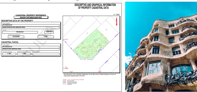
Figure1: An example of building information contained in the Cadaster: La Pedrera
CADASTRAL PROPERTY REFERENCE
0032917DF3803C0001WZ
DESCRIPTIVE DATA OF THE PROPERTY
POSTAL ADDRESS PS GRACIA 92 08008 BARCELONA [BARCELONA] MAIN USE Residential CONSTRUCTION YEAR 2017 PARTICIPATION COEFFICIENT 100,000000
TOTAL BUILT SURFACE ]m²
11.861
CA'ASTRAL3$5&(/
POSTAL ADRESS
PS GRACIA 92 BARCELONA [BARCELONA]
TOTAL BUILT SURFACE ] 11.861
GRAPHICAL PARCEL SURFACE ]m²
1.808
TYPE OF PROPERTY
DESCRIPTIVE AND GRAPHICAL INFORMATION OF PROPERTY CADASTRAL DATA
E: 1/800
4,582,950 4,583,000
429,900 429,950
429,950 U.T.M. coordinates Zone 31 ETRS89
7KLVGRFXPHQWLVQRWDFDGDVWUDOFHUWLILFDWLRQEXWLWVGDWDFDQEHYHULILHGWKURXJKWKH$FFHVVWR XQSURWHFWHGFDGDVWUDOGDWDRIWKH6(&.
Block boundary Land parcel boundary Buildings boundaries Sidewalks CONSTRUCCIÓN
Destino Escalera Planta Puerta Superficie m² PUBLICO C OM UN 1.274 PUBLICO -1 01 230 PUBLICO -1 02 28 PUBLICO -1 03 84 PUBLICO -1 O1 290 PUBLICO -1 O2 85 PUBLICO -1 04 40 PUBLICO 0 04 63 PUBLICO -1 05 63 PUBLICO 0 01 135 PUBLICO 0 02 75 PUBLICO EN 01 714 PUBLICO 0 03 67 PUBLICO 0 05 39 PUBLICO 0 06 68 Continúa en ANEXO I
1906-1912
Source:http://www.sedecatastro.gob.es(left image). Photo byFlorencia Potteronunsplash.com(right image).
All unprotected data referring to each property, identified by its cadastral reference, can
be downloaded from the Cadaster at http://www.sedecatastro.gob.es. These data include
all information about the building except that referring to its ownership and value. For each building, this url provides access to an online form that provides basic information and which can be downloaded in PDF format. It also gives access to a detailed map of the building that can be downloaded in GIS format and detailed information about such characteristics as:
1) the building’s exact location and total built surface, 2) the year of construction, 3) its use
(residential or non-residential), 4) height (number of floors above ground), 5) its footprint (m2),
1
and6) the number of total units that are contained in each building and, specifically, the number
of residential units (dwellings). By way of illustration, Figure 1 shows the online form and
footprint map of Antoni Gaud´ı’s well-known building, ‘La Pedrera’, in Barcelona. The online
form indicates that it was built between 1906and1912, and records its postal address, footprint
(1.808km2) and main use (residential).
Table 1 reports the main figures to be drawn from the database. Thus, in Spain there are
more than12 million buildings (that is,0.25buildings per capita;75% of them with a residential
use) made up of just more than 37 million units (63% of which are classified as dwellings). As
discussed in the Introduction, it is especially useful to exploit the information available about building heights and footprint to obtain what we denote as the ‘horizontal’ area (the building’s footprint) and the ‘vertical’ area (which is obtained by multiplying the building’s footprint by the
number of floors). The horizontal area of the buildings in Spain covers3,099km2(less than1% of
the country’s total surface area), while the vertical area is nearly three times that of its horizontal
area (8,468km2), which corresponds roughly to the average height of three floors per building.
Table1: Buildings in Spain
Counts Areas
Buildings 12,069,635 Horizontal area =∑(Building footprint) 3,099km2
Residential 75.7% Percentage of Spain’s land area 0.6%
Non-residential 24.3%
Units within buildings 37,011,784 Vertical area =∑(Footprint×floors) 8,468km2
Residential 63.3% Residential 65.2%
Non-residential 36.7% Non-residential 34.8%
Average number of floors 2.9
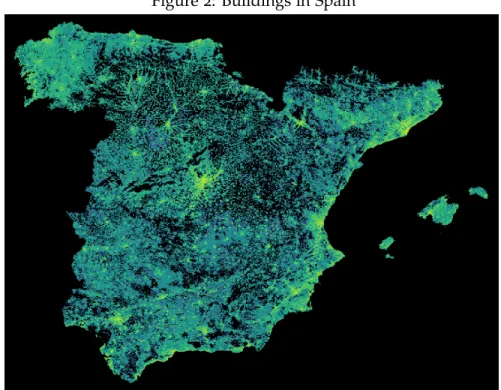
Figure2: Buildings in Spain
Figure2shows the distribution of buildings across Spanish territory (the colored dots reflecting
and yellow dots indicate areas with an increasing concentration of buildings (with yellow showing the highest concentrations). The areas with most yellow dots appear along the Spanish coast and in the center of the country, with the Madrid area being the brightest.
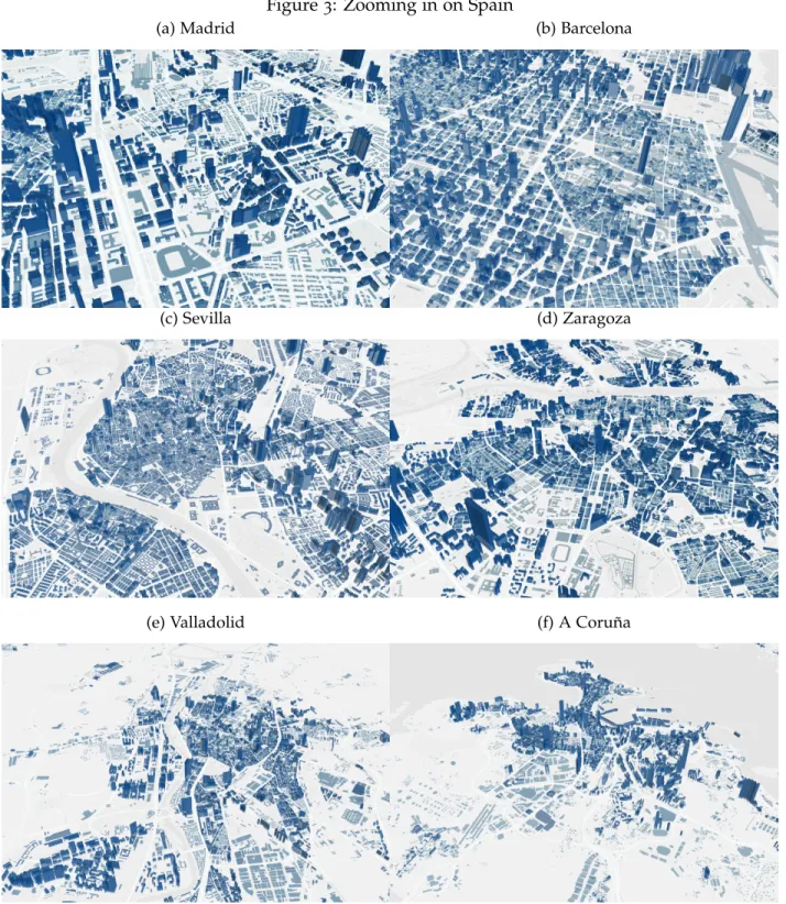
Figure3 presents3-D illustrations of the location of buildings in central areas of the
present-day municipalities of Madrid, Barcelona, Sevilla, Zaragoza, Valencia and A Coru ˜na. Interestingly, the concentration of buildings and the verticality of these areas is quite distinct.
Figure3: Zooming in on Spain
(a) Madrid (b) Barcelona
(c) Sevilla (d) Zaragoza
3. Delineating urban areas with buildings and a machine learning algorithm
We delineate urban areas as portions of land with a minimum, uninterrupted level of building density. To do so, we develop a novel approach as an extension of a well-understood
ma-chine learning algorithm (DBSCAN; Ester et al., 1996) that we name ‘Approximate DBSCAN’
(A-DBSCAN)2
. Its purpose is to detect robust clusters of buildings that reach a minimum density threshold. To achieve this, our algorithm requires two input parameters: first, the minimum number of buildings that each urban area (cluster) needs to include to be considered so; and, second, a maximum search distance in which to count surrounding buildings to check whether the first criterion is satisfied. Once a set of buildings is identified as a cluster, our method draws
its surrounding boundary using theα-shape algorithm Edelsbrunner et al.(1983), a widely used
approach to delineate tight bounding boxes.
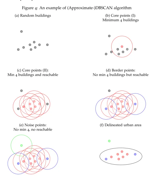
Figure 4 illustrates how DBSCAN works for a random group of buildings (Figure 4a) when
the minimum number of buildings is set at four. The algorithm first chooses a building (in red), draws a circle with a radius equal to the chosen distance threshold (the second parameter) and
evaluates the minimum number criterion (Figure4b). In this case, the criterion is satisfied and this
building is labelled as a ’core’ point. The algorithm continues to run by drawing circles around
the other points and evaluating the minimum number criterion. Figure4cshows all the buildings
that satisfy the minimum number criterion and which are core points. All these buildings/points are reachable, that is, there is a direct connection from one building to another or an indirect link via paths that cross through other core buildings.
Figure4d shows other buildings (in blue) that do not satisfy the minimum number criterion
but which are reachable from some core buildings (i.e. they are within the core building circles). These are the so-called ‘border’ points and they also belong to the delineated urban area. Finally,
Figure 4eshows a building (in green) which, after drawing the circle with a radius equal to the
distance threshold, does not satisfy the minimum number criterion. This type of building/point is the so-called ’noise’ point and does not belong to the delineated urban area.
The final delineated urban area (Figure4f) is made up of core and border buildings (red and
blue points) but does not include any noise buildings (green points). By definition, the core of the delineated urban area has the highest density of buildings and the border area the lowest. As a result, our definition of the urban area is in line with the traditional idea of a city, that is, a place with high levels of building density and with an urban spatial structure in which building density decreases towards its the boundaries.
When applying the algorithm to our building dataset, we set the two parameters – that is, the minimum number of buildings and the distance threshold – based on knowledge and evidence
from the Spanish urban system. First, we set the minimum number to 2,000buildings in order
to ensure the urban areas we delineate house, at least, 5,000 people. On average, the Spanish
household comprises 2.5 members (Instituto Nacional de Estad´ıstica, 2018). This minimum
threshold is set assuming that the average building is a single family house, which is not exactly
2
An open-source implementation of A-DBSCAN, written in Python following thescikit-leanAPI, is available at
the case of some areas of Spain. However, we do not want to underestimate, or rule out altogether, the newer settlements built largely in accordance with that model of urban development. For the
maximum distance threshold, our preferred results use2,000m. This parameter is chosen based
on information about Spanish commuting patterns. The average daily distance commuted by a
person in Spain’s biggest cities is approximately 4 km (Cascajo et al., 2018) which, divided by
two, yields2km per trip.
Figure4: An example of (Approximate-)DBSCAN algorithm
(a) Random buildings (b) Core points (I): Minimum4buildings
(c) Core points (II): Min4buildings and reachable
(d) Border points:
No min4buildings but reachable
(e) Noise points: No min4, no reachable
(f) Delineated urban area
As mentioned, our approach uses a machine learning algorithm, based on the original
DB-SCAN developed by Ester et al. (1996). DBSCAN facilitates cluster identification based on
measures of density without the need for auxiliary geographies. However, from a computational point of view, it does not scale well and, more importantly, it does not include any mechanism to ensure the robustness of the clusters (or, in our case, urban areas). To address this shortcoming,
we specifically developed the A-DBSCAN extension. Thus, we propose turning the original
algorithm into an ensemble that combines a number of exact DBSCAN runs (1,000replications)
on random subsamples (10% of the original dataset) that are expanded to the rest of the sample
through a nearest-neighbor algorithm. These solutions are then summarized in one final set of urban areas (clusters) in which buildings are classified based on their most common occurrence. That is, to ensure robustness, the buildings belonging to an urban area are those assigned to
that urban area in at least 90% of the replications. Otherwise, these buildings are classified as
noise points and do not belong to any urban area. A more detailed and technical explanation of
A-DBSCAN is provided in AppendixA.
We perform several experiments to explore the degree of agreement between our algorithm and the original DBSCAN. An ideal test in this context would be to compare the results of the two algorithms when applied to the entire dataset of Spanish buildings. However, this is not computationally feasible (indeed, one of the reasons for the development of A-DBSCAN is precisely to overcome this computational hurdle). Instead, we consider different parts of Spain characterized by varying numbers of buildings and population, urban areas of different size, and by different geographical features. We are then able to run both algorithms on these subsets and
to compare their delineated urban areas. To do so, we use the ‘adjusted Rand index’ (Hubert and
Arabie, 1985), a measure of similarity between two groups or classifications that is widely used in machine learning. In our case, we compare the set of delineated urban areas and the buildings
that make up each area when using (1) our algorithm (with the 1,000 replications) and (2) the
original DBSCAN. Mathematically,
Rand index= a+b
a+b+c+d
where a is the number of buildings that are assigned to the same urban areas in (1) and (2);bis
the number of buildings that are assigned to different urban areas in (1) and (2);cis the number
of buildings that are assigned to the same urban areas in (1) and to different urban areas in (2);
dis the number of buildings that are in different urban areas in (1) and in the same urban areas
in (2). Intuitively,a+bcan be considered as the number of agreements (i.e., buildings assigned
to the same urban areas in (1) and (2)) andc+das the number of disagreements (i.e., buildings
assigned to different urban areas in (1) and (2)). As a result, the Rand index measures the ratio
of agreements between the two methods over the total number of buildings, and its values range
between0, dissimilarity, and1, maximum similarity3.
The first three columns in Table 2 present the results of these comparisons for six different
parts of Spain. Column 1 shows their geographical location; column 2 reports the size of their
population, and column 3 presents the corresponding Rand index. In general, the degree of
similarity between the delineated urban areas when using the two methods is quite high, with the
maximum value being recorded for Sevilla (with a97% degree of similarity)4. This is remarkable
because our algorithm uses only 10% of the entire sample to calculate the exact DBSCAN (with
3
We use the adjusted version of this index that corrects for the probability of buildings being assigned to the same urban areas by chance. To do so, we use the implementation in the Python libraryscikit-learn(Pedregosa et al.,
2011).
4
1,000replications), and then extrapolates the structure captured in that subset to the rest of the
dataset. Altogether, these results provide evidence of the efficiency and effectiveness of our algorithm.
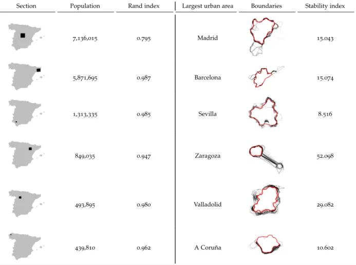
Table2: A-DBSCAN
Section Population Rand index Largest urban area Boundaries Stability index
7,136,015 0.795 Madrid 15.043 5,871,695 0.987 Barcelona 15.074 1,313,335 0.985 Sevilla 8.516 849,035 0.947 Zaragoza 52.098 493,895 0.980 Valladolid 29.082 439,810 0.962 A Coru ˜na 10.602
Notes: Gridded population data from National Institute of Statistics (INE).http://ine.es/censos2011_datos/cen11_datos_ resultados_rejillas.htm
An additional advantage of our algorithm is its sampling approach, since it allows us to explore the stability of the delineations. In other words, given that each of the final delineated urban areas
are based on1,000replications, it is possible to quantify the degree of agreement between the1,000
delineations for each urban area. The last three columns in Table2explore this dimension for the
largest urban areas (column 4) found in each of the aforementioned parts of Spain. In column5
we draw the final boundaries of each urban area (the thicker red line) on top of the delineations of each replication (thinner black lines). The figures allow us not only to compare the overall stability between delineations, but also to identify areas within a given urban area of greater and lesser stability. For instance, while A Coru ˜na’s northern side displays a high degree of agreement, its southern border is more variable across replications, suggesting a more nuanced boundary. This approach also identifies borderline cases associated with more disperse developments that meet the requirements imposed by the algorithm in a large number of replications but not in enough
to grant final assignation into the urban area. Zaragoza is a good example of this situation. To summarize these visual displays, we compute a Stability index, which is based on the average difference between the delineated area in each single replication and that of the final delineated urban area. We express its value as a percentage of the final surface to correct for city size effects: Stability index=
∑
r |Ar−A˚| R 100 ˚ Awhere Ar is the surface of the boundary obtained in replication r, ˚A is the surface of the final
delineation, and Ris the total number of replications. This measure captures the extent to which
individual boundaries drawn as part of our method spatially overlap with the final boundary chosen. Each individual drawing of the boundary might be larger than the final one (as illustrated
in the visualizations in Table2) and include buildings that do not form part of the final delineated
urban area. However, the difference between the two offers a measure of the stability of the final delineation and of the extent to which urban development is clearly delimited in the periphery of an urban area or, on the contrary, the degree to which it fades away progressively. The index has a lower bound of zero for the case of complete stability, when all replications agree exactly, and is not upper bounded (the difference between the final delineation and each replication can be
arbitrarily large). Column 6 in Table2 reports the Stability indexes for the selected urban areas.
In general, the values show high degree of stability in the delineations. Once again, the case of Sevilla stands out as it shows the closest value to zero and, as a result, the highest degree of stability between the delineations. In contrast, and as mentioned when discussing the boundaries
(column 5), less stability is found in Zaragoza because of a disperse development that is not
assigned to the final delineation of its urban area.
In summary, our algorithm for delineating urban areas has certain advantages over other methods. First, it is density-based and, in combination with our building dataset, identifies urban areas that only contain continuous parcels of space where the building density exceeds a minimum threshold. As discussed, this feature is in line with the traditional idea of a city that has come into existence because of the agglomeration economies created by the high concentration of population and firms. On the other hand, delineations based on, for example, commuting and/or administrative boundaries include large areas of undeveloped land, which reduces the overall city density. Second, our delineated urban areas are spatially continuous collections of buildings rather than exogenous aggregations, such as grid cells or administrative boundaries. Such ex-ante groupings may be necessary when there is no information available about individual locations or even justified in some specific cases but, generally, they imply a loss of granularity. Furthermore, they can potentially distort the final conclusions of analyses based on them: the
so-called ‘Modifiable Areal Unit Problem’ (MAUP) (Openshaw, 1984, Briant et al., 2010). Third,
our algorithm is robust to marginal changes in the data and has a “built-in” approach to explore solution stability. Furthermore, similar to bootstrap estimates, the proposed sampling approach ensures the results are computationally scalable and, thus, feasible in large datasets like ours
4. Urban areas in Spain
4.1 Main results
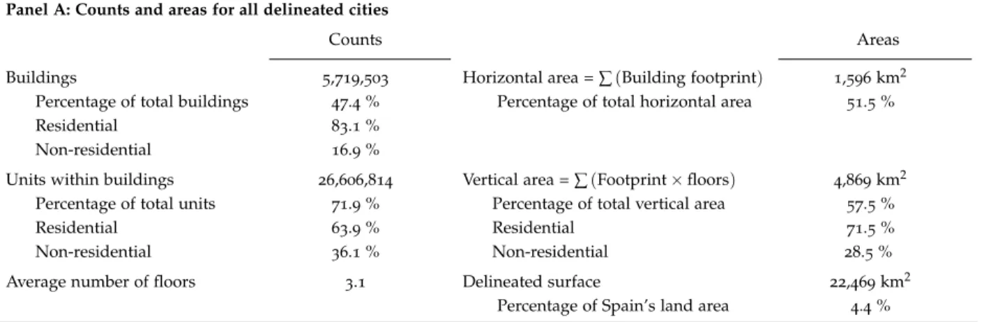
As can be seen in Table3, our method delineates717urban areas that account for approximately
75% of the Spanish population. These areas contain5.7million buildings (roughly half of Spain’s
total), made up of 26 million units (72% of the total). The sum of building footprints (the
horizontal area) is 1,596 km2. When we also take into account the buildings’ floor area (the
vertical area), this figure is multiplied by three (4,869km2). Interestingly, the average number of
floors in the buildings in these urban areas is three. When considering the buildings’ footprint together with the land lying between the buildings (streets, roads, parks, etc.), the total surface
of the delineated urban areas reaches22,469km2, which represents nearly5% of the surface area
of the whole of Spain. The use of the buildings of these urban areas is mainly residential (83.1%
of the cases). As for the population size of the delineated urban areas (Table 3 Panel B), ten
of them have more than 500,000inhabitants and represent one third of the Spanish population.
Together with the next 47 biggest urban areas (those with a population between 100,000 and
500,000inhabitants), they represent52% of the whole Spanish population. The data for these ten
urban areas seem to indicate that the biggest ones in terms of population have larger surfaces and vertical lands. For the delineated urban areas, the correlation between their population and
surface is 0.89, while that between their population and vertical land is even bigger (0.98).
Table3: Buildings and delineated urban areas
Panel A: Counts and areas for all delineated cities
Counts Areas
Buildings 5,719,503 Horizontal area =∑(Building footprint) 1,596km2
Percentage of total buildings 47.4% Percentage of total horizontal area 51.5%
Residential 83.1%
Non-residential 16.9%
Units within buildings 26,606,814 Vertical area =∑(Footprint×floors) 4,869km2
Percentage of total units 71.9% Percentage of total vertical area 57.5%
Residential 63.9% Residential 71.5%
Non-residential 36.1% Non-residential 28.5%
Average number of floors 3.1 Delineated surface 22,469km2
Percentage of Spain’s land area 4.4%
Panel B: Number of urban areas by population size
Urban areas Population Percentage of Spain’s pop
All 717 35,015,936 74.8% Population≤5,000 131 472,080 1.0% 5,000<Population≤10,000 220 1,566,350 3.4% 10,000<Population≤25,000 189 2,971,230 6.4% 25,000<Population≤100,000 120 5,719,630 12.2% 100,000<Population≤500,000 47 8,742,245 18.7% Population>500,000 10 15,544,400 33.2%
Notes: In2011,46,815,916inhabitants lived in Spain. Population is computed using population grid data (1×1km cells within the
These results are obtained when the algorithm considers the number of buildings to be
found within a 2,000-meter threshold. However, we also calculated the algorithm modifying
this distance to see how it affects our results. Table B.1 in Appendix B presents the results of
the delineated urban areas with different distance thresholds (1,500m, 1,600m, 1,800m, 2,200
m,2,400m and 2,500m). As expected, as the threshold distance falls, the number of delineated
urban areas increases and the percentage of population contained in the new delineated urban
areas diminishes. Thus, for the smallest distance threshold (i.e. 1,500 m), we obtain 773urban
areas (with 70% of the population). In contrast, as the distance increases, we obtain fewer urban
areas containing more population. For example, when the distance was greatest (i.e. 2,500m),
699urban areas are delineated containing79% of the total Spanish population.
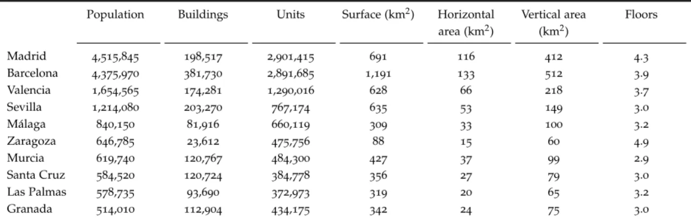
Table4describes the characteristics of the ten largest urban areas in Spain in terms of
popula-tion, number of buildings and units, surface, horizontal and vertical area and number of floors. It is interesting to see the different structures presented by these urban areas. For example, Madrid
and Barcelona contain a similar number of inhabitants (4.52M and 4.37M, respectively) but the
surface area and the number of buildings they contain is quite different. Barcelona has nearly twice the surface area and twice the number of buildings as Madrid. The other eight urban areas are much smaller.
Table4: The largest delineated urban areas
Population Buildings Units Surface (km2) Horizontal
area (km2) Vertical area (km2) Floors Madrid 4,515,845 198,517 2,901,415 691 116 412 4.3 Barcelona 4,375,970 381,730 2,891,685 1,191 133 512 3.9 Valencia 1,654,565 174,281 1,290,016 628 66 218 3.7 Sevilla 1,214,080 203,270 767,174 635 53 149 3.0 M´alaga 840,150 81,916 660,119 309 33 100 3.2 Zaragoza 646,785 23,612 475,756 88 15 60 4.9 Murcia 619,740 120,767 484,300 427 37 99 2.9 Santa Cruz 584,520 120,724 384,778 356 27 79 3.0 Las Palmas 578,735 93,690 372,973 319 20 65 3.2 Granada 514,010 112,904 434,175 342 24 75 3.0
Notes: Population is computed using population grid data (1×1km cells within the boundaries of our urban areas) from the2011
Population Census. Surface is total land of the delineated urban area. Horizontal area refers to the sum of building footprints. Vertical area is the sum of floor footprints. Floors refers to the average number of floors.
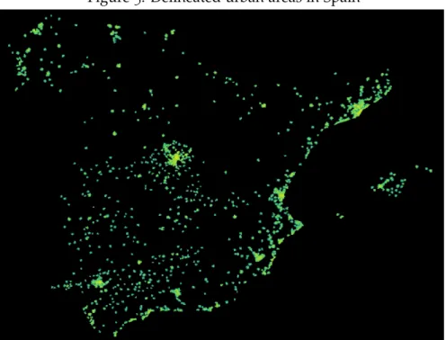
Figure 5 shows the geographical location of the 717 urban areas (with colors ranging from
green to yellow with increasing density of buildings within the urban area). As can be seen, most of the urban areas are concentrated along the Mediterranean coast, and in the center and south
of Spain. The smaller scale illustration in Figure6shows the delineated urban areas in the region
of Barcelona.
It is interesting to compare our results with those reported byBellefon et al. (2019) who also
delineate the French urban areas using building density but the authors apply a new dartboard methodology. Although France and Spain are similar countries (in terms of economic develop-ment, location, etc.), some aspects of their respective urban structures differ considerably. France
per capita (covering just0.6% of the territory). Likewise, the average number of floors in French
buildings is two, while, as we have seen, in Spain it is three. Thus, initially it would appear that France presents a less dense urban system. When applying the delineation method to French
buildings,7,223urban areas are obtained of which695have a core. These areas concentrate75%
of the French population. This last figure is quite similar to the one reported here for the Spanish urban areas.
Figure5: Delineated urban areas in Spain
4.2 Identifying employment centers within the urban areas
An interesting exercise to illustrate a further application of our method is the identification of employment centers within each of the urban areas. The goal of this exercise is to focus specifically on the concentration of economic activity. With this purpose in mind, we adopt a
similar approach to that described in Section3, albeit with some differences. Most importantly,
we focus on units rather than on buildings, given that a single building may include several units (especially if it contains more than one floor). This is a prevalent feature of CBDs and other forms of employment concentration where firms and workers cluster to benefit from density. Using units instead of buildings also allows us to account for the difference between vertically dense areas and those clustered only horizontally. This implies, in the case of this exercise, working only with the non-residential units.
Although the identification mechanism is similar to that used when delineating city bound-aries, a few changes have to be introduced. First, instead of running a single instance of the algorithm for the entire dataset, we apply the method to each urban area delineated in the previous stage. Second, for each dataset of urban area buildings, we run A-DBSCAN using
50% of the sample. We retain 90% as the stability threshold and 1,000 replications to generate
the delineations. Third, while each point still represents a single building, we now weight them based on the number of non-residential units that the building houses. Finally, we adapt our two algorithm parameters (minimum number of buildings per urban area and distance threshold) to identify employment centers in accordance with methods proposed in the literature. The
most frequently used are those based on density thresholds (Giuliano and Small,1991,McMillen
and Smith, 2003, Giuliano et al., 2007, Mu ˜niz et al., 2008) and density peaks (McMillen, 2001,
Redfearn, 2007, Garcia-L ´opez et al., 2017b,a), where an employment center is a place whose primary feature is a high density of workers (and certainly one with a density higher than that of
nearby locations).Giuliano and Small(1991) andMcMillen and Smith(2003) define this density as
2,500employees per km2. Assuming ten employees per non-residential unit (Fari ˜nas and Huergo,
2016), the threshold we need to impose is 250 non-residential units per km2. By considering a
distance threshold of250m, the minimum number of non-residential units is therefore495.
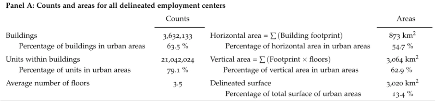
Table 5 presents the results of the delineation of the employment centers within each of the
urban areas. Panel A shows that the footprint of the employment centers amounts to 886 km2
(that is, 55% of the horizontal land of all the urban areas). Interestingly, the economic activity
inside the urban areas is clearly more concentrated and presents a distinct pattern of location to that of residential use. When we analyze the vertical land associated with these employment
centers, the surface increases to3,060km2(that is,63% of the vertical land of all the urban areas).
Thus, unsurprisingly, insofar as the average number of floors is 3.5 in the employment centers,
the density of buildings in these areas is higher.
Panel B shows that, with no restriction on the size of the employment centers, the717urban
areas contain2,056employment centers. However, when we establish a minimum number of jobs
per center (so as to take the largest economic agglomerations into consideration), the number of
5
Since the circle around each unit has an area of0.196km2 (=(0.250)2×π), the minimum number of units can be
employment centers falls. Thus, there are only70employment centers with more than10,000jobs
and just seven centers with more than50,000jobs. In fact, only the biggest urban areas have more
than one employment center with more than10,000jobs. This is the case, for example, of the cities
of Barcelona (nine employment centers), Valencia (five), Madrid (four) and M´alaga (three). This evidence is in line with the polycentric structure of these urban areas as reported and analyzed by (Garcia-L ´opez, 2010, 2012). To illustrate how the algorithm works to delineate employment
centers at a smaller scale, Figure7shows the nine biggest delineated centers in the urban area of
Barcelona.
Table5: Delineated employment centers in the urban areas
Panel A: Counts and areas for all delineated employment centers
Counts Areas
Buildings 3,632,133 Horizontal area =∑(Building footprint) 873km2
Percentage of buildings in urban areas 63.5% Percentage of horizontal area in urban areas 54.7%
Units within buildings 21,042,024 Vertical area =∑(Footprint×floors) 3,064km2
Percentage of units in urban areas 79.1% Percentage of vertical area in urban areas 62.9%
Average number of floors 3.5 Delineated surface 3,020km2
Percentage of total surface of urban areas 13.4% Panel B: Number of employment centers by size
Employment centers Urban areas
All 2,056 in 717 Employment≤2,500jobs 1,420 in 503 2,500<Employment≤5,000 347 in 297 5,000<Employment≤10,000 193 in 169 10,000<Employment≤25,000 70 in 63 25,000<Employment≤50,000 19 in 17 Employment>50,000 7 in 7
5. Comparing our delineated urban areas
Comparing our urban area delineation results, obtained with a machine learning method based on the geolocation of the country’s buildings, with previous delineations performed for Spain is far from straightforward. The main reason for this is that all previous methodologies have taken the municipality (i.e. the political administrative local entity) as their starting unit of analysis. In such studies, urban areas were built by aggregating surrounding municipalities to a central
one. Spain has8,131municipalities, most of them quite small (in fact,90% have fewer than5,000
inhabitants) and with considerable variation in terms of their surface area. This suggests that these methodologies are likely to be much less precise and that their results cannot be treated at the same scale as ours. Despite this, it is nevertheless interesting to compare our results with those obtained using these different methodologies.
In recent years, there have been a few attempts to aggregate municipalities into urban areas.
The Statistical Atlas of Urban Areas (Atlas Estad´ıstico de las ´Areas Urbanas), published at fairly
regular intervals, by the Ministry of Public Works defines91urban areas. The main limitation of
the methodology employed, besides its use of the administrative borders of the municipalities as
its starting unit, is that it only considers an urban area if the central city has more than 50,000
inhabitants. After identifying these big central municipalities, neighboring municipalities with sufficient economic links and sufficient numbers of commuters between the two units are added. Employing a very similar methodology, the AUDES research Project (AUDES Areas Urbanas
de Espa ˜na6
), conducted in 2010, represented another attempt to delineate urban areas. The
aim of this project was to delineate all the urban areas in Spain (not just the biggest ones)
using commuting and urban contiguity patterns. As a result, 261 urban areas were defined.
The restriction imposed by the AUDES project was that an urban area had to have a minimum
population of20,000inhabitants.
Addressing a different objective, and drawing solely on commuting data from the2011Census,
Feria and Mart´ınez-Bernab´eu (2016) defined Local Labor Markets for Spain by adapting the
procedure employed by the Office of Management and Budget for the US Census7
. The main limitation of this particular exercise was that the initial population threshold imposed by the
authors was100,000inhabitants and for this reason they identified just41local labor markets.
As discussed, comparing our urban area delineations with existing ones is conceptually
challenging but empirically possible. By way of an initial approach, Panel B in Table 6 ranks
the 10 largest urban areas delineated by the AUDES methodology that we consider to have the
fewest limitations, as well as being the one for which we can access most data. We include our results in Panel A and, in Panel C, the outcomes corresponding to the municipalities’ administrative borders, which we consider informative. For each urban area and method, we
show the population (in thousands of inhabitants), the surface (in km2) and the vertical area (in
km2).
6
AUDES project. Documentation and open data available at http://alarcos.esi.uclm.es/per/fruiz/audes/
(accessed March2018).
7
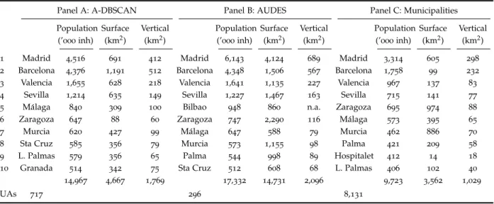
Table6: Main urban areas identified in Spain using different delineation methods
Panel A: A-DBSCAN Panel B: AUDES Panel C: Municipalities Population (’000inh) Surface (km2) Vertical (km2) Population (’000inh) Surface (km2) Vertical (km2) Population (’000inh) Surface (km2) Vertical (km2) 1 Madrid 4,516 691 412 Madrid 6,143 4,124 689 Madrid 3,314 605 298 2 Barcelona 4,376 1,191 512 Barcelona 4,348 1,506 567 Barcelona 1,758 99 232 3 Valencia 1,655 628 218 Valencia 1,641 1,135 227 Valencia 967 137 83 4 Sevilla 1,214 635 149 Sevilla 1,227 1,467 163 Sevilla 715 141 77
5 M´alaga 840 309 100 Bilbao 948 860 n.a. Zaragoza 695 974 88
6 Zaragoza 647 88 60 Zaragoza 747 2,290 116 M´alaga 573 395 65
7 Murcia 620 427 99 M´alaga 647 588 79 Murcia 462 886 70
8 Sta Cruz 585 356 79 Murcia 573 1,155 98 Palma 421 209 58
9 L. Palmas 579 356 65 Palma 544 998 89 Hospitalet 412 14 18
10 Granada 514 342 75 Sta Cruz 512 608 68 L. Palmas 406 102 40 14,967 4,667 1,769 17,332 14,731 2,096 9,723 3,562 1,029
UAs 717 296 8,131
On average, a comparison of our delineations with those performed by AUDES shows that
our method delineates cities that contain less population (up to15% less). Likewise, the pattern
that emerges when considering area as opposed to population is similar, and if anything slightly more restricted boundaries than those identified by AUDES (our urban areas have a surface area that is one third less). Indeed, proportionally, these differences are larger than when considering population. This outcome is probably the consequence of our working with buildings instead of basing the aggregation on the municipal units. However, it is interesting to see how this approach affects some of the biggest urban areas. For example, while the population assigned to
Madrid’s urban area by AUDES is40% greater than that delineated by our algorithm (6.1vs4.5M,
respectively), the area within the city’s boundary is almost seven times larger for AUDES than
for our delineation (4,124vs 691 km2, respectively). In the case of the urban area of Barcelona,
the outcome is quite distinct. Both methods delineate an area of similar population (around4.3M
inhabitants) but the surface assigned by AUDES is 26% greater than that assigned when using
our method (1,506vs1,191km2). Interestingly, the surface of the administrative area of Barcelona
is just 99 km2. In contrast, the urban areas of Zaragoza and Murcia are especially extensive
according to the administrative delineation of their borders (974 and 886 km2, respectively),
but their surface sizes are much smaller according to our delineation method (88 and427 km2,
respectively). As for the vertical land of the urban areas, even this is greater, on average, according to the AUDES delineation, although the difference between the two methods is smaller than that for their respective surface areas.
Because our method takes buildings as its basic unit of analysis and does not impose any ancil-lary geography to calculate densities, the boundaries it generates do not include any low density spaces, which abound in the peripheries of Spain’s municipalities. However, it should be borne in mind that these conclusions are based on a small subset of cities. To provide confirmation, we would need to expand the analysis to the entire set of delineations. In the sections that follow, we report different exercises aimed at comparing more accurately the outcomes of the different delineation methods.
5.1 Rand index and overlapping
In this section, we employ the adjusted Rand index (see Section 3) to compare our delineated
urban areas with those of the AUDES project and the Spanish municipalities. As discussed,
the index developed by Hubert and Arabie (1985) measures the ratio of agreements (buildings
assigned to the same urban area in two delineations) over the total number of buildings, and its
values range from0, dissimilarity or no overlap, to 1, maximum similarity or complete overlap.
The ratio between our algorithm and AUDES is 0.350, while that with the municipalities is
0.003, indicating that the former provides the closest definition to our own delineations, while
the municipalities is least similar8
.
Another way to compare the three delineations is simply by analyzing the extent to which, and just where exactly, the alternative delineations (AUDES and municipalities) are included
within the boundaries defined by our algorithm. Figure 8 presents two histograms showing
the number of AUDES urban areas and Spanish municipalities included within our A-DBSCAN
boundaries (Figures 8a and 8c, respectively) and two maps showing their location (Figures 8b
and 8d, respectively). In line with the evidence presented in the paragraph above, A-DBSCAN
delineations coincide much more closely with the AUDES boundaries than they do with the municipalities. This is to be expected, given that AUDES are groups of municipalities linked by their common geography and commuting flows. However, the figure provides evidence that our method is able to approximate these same boundaries using a quite distinct approach.
Geographically, our maps also reveal a number of clear patterns. Our delineated urban areas containing parts of more than two AUDES are disproportionately located in the Mediterranean coast. We interpret this in terms of the type of urban development present in this region compared to that in the rest of Spain. The Mediterranean region is much more developed than the rest of the country. The density of urban development is also much higher, as can be discerned from
Figure 2. This pattern results in A-DBSCAN identifying larger contiguous areas in which the
building density is above the threshold required for an area to be considered urban. In turn, this makes our definitions of Barcelona, Valencia, or Alicante, among others, larger than their AUDES counterparts. In contrast, in the center of the country, a much sparser region with well delimited towns and cities, most urban areas delineated by A-DBSCAN contain only one AUDES.
8
The index between AUDES and municipalities is 0.007and, as a result, the degree of similarity between both
Figure8: Overlap between different urban area delineations
Panel A: AUDES urban areas included in A-DBSCAN delineations.
(a) (b)
Panel B: Municipalities included in A-DBSCAN delineations.
(c) (d)
5.2 City size distribution
Zipf’s law suggests that a country’s city size distribution can be approximated with a Pareto distribution with shape parameter equal to one. The higher (lower) the Pareto exponent, the more equally (unequally) distributed is the city system. The power law implies that, in a system of cities, the largest city is roughly twice the size of the second largest city, about three times
the size of the third largest city, and so on. Indeed, since the seminal work ofGabaix (1999) and
Eeckhout(2004), an enormous amount of city size distribution literature has been published (see
The evidence reported by this literature is mixed. In some cases the law holds precisely but, in others, the outcome lies some distance from the unit parameter. The variety of results seems to be attributable to the city definition employed and, as a consequence, to the heterogeneity in the city samples used to perform the tests. Given this situation, it is interesting to compare the
city size distribution by simulating an exercise performed by Rozenfeld et al. (2011) in which
different definitions of city within the same country are taken into consideration. Thus, in the following paragraphs, we seek to determine whether the city size distribution in Spain depends on the definition of the units of analysis.
Figure 9 plots the log-ranks against the log-sizes for the urban area boundaries created by:
1) our algorithm A-DBSCAN, 2) AUDES commuting-based patterns, and 3) the administrative
municipalities. Panel A shows the plots for the three delineations using population as the measure
of each urban area’s size9
. The estimated Pareto exponent is negative and very close to1for both
our delineated urban areas and those from the AUDES project (-0.97 and -0.99, respectively). As
discussed above, if the estimated value of the Pareto exponent is equal to one, then Zipf’s law is confirmed as holding exactly for these two delineations. In contrast, the estimated parameter
for the administrative municipalities is -1.23, indicating that Zipf’s law does not fit in this case
and also that the distribution of the population across these units is more unequal. However, the
relationship does fit the log-linear specification quite well in all three cases (with an R2 of 0.99,
0.99and 0.88, respectively). Interestingly, in all three delineations the slope fits very well in the
upper tail of the distribution.
Most of the evidence tests Zipf’s law by comparing city sizes and their populations (with the
notable exception ofRozenfeld et al.,2011). However, our data allow us to replicate the analysis
using the surface (Panel B) and the vertical land (Panel C) of the urban areas. In the case of the former, our results indicate that Zipf’s law holds only for the urban areas produced by our
delineation (with an estimated Pareto exponent of -1.09 and an R2 of 0.98). Interestingly, for
the bigger urban areas (the upper tail of the distribution) the linear fit is not perfect. For the AUDES urban areas and the municipalities the estimated values for the coefficients lie far from
the unit (-0.78and -0.61, respectively) and the R2 values are smaller (0.79 and0.61, respectively).
In both cases, the slopes show a log-quadratic, as opposed to a log-linear, relationship between surface-rank size. When the size of the urban areas is measured in terms of the vertical land (Panel C), the estimated coefficients for both our urban delineated areas and the AUDES areas are very
close to -1 (-1.04 and -1.09, respectively). In the case of the municipalities, whose distribution
presents a clear concave shape, the coefficient is -0.67clearly indicating that Zipf’s law does not
hold for this delineation. A detailed inspection of the shape of the distribution of the AUDES urban areas shows that the biggest city in terms of vertical land is a clear outlier. This is not the case for our delineated urban areas, which present a more continuous pattern.
9
The AUDES delineation only reports urban areas with more than20,000inhabitants. For the comparisons to be
Figure9: Zipf plots for different measures of city size
Panel A: Population
A-DBSCAN AUDES Municipalities
Panel B: Surface
A-DBSCAN AUDES Municipalities
Panel C: Vertical
A-DBSCAN AUDES Municipalities
5.3 City size and transportation
As has been well documented, one of the main problems urban economists face is the so-called
’Modifiable Areal Unit Problem’ (MAUP) (Openshaw,1984). AsBriant et al.(2010) have shown,
empirical results can change when different spatial units are adopted. In this subsection, we compare our delineated urban areas with AUDES urban areas and Spanish municipalities by
studying how city size relates to transportation10
.
Based on empirical studies analyzing the impact of transportation on city size measured in
terms of population (Duranton and Turner, 2012, Garcia-L ´opez et al., 2015, Garcia-L ´opez et al.,
2018, Baum-Snow et al., 2019) and land area (Brueckner and Fansler,1983, Garcia-L ´opez, 2019), we can estimate the following equation:
ln(City size) =α0+
∑
i
(α1,i×ln(Transportationi)) +
∑
j
(α2,j×Controlsj) (1)
We consider three dependent variables to measure city size. First, in line with tradition,
we consider the size of the city in terms of population using the log of the 2010 population
(inhabitants). Second, we take into account the physical size of the city’s surface, that is, its size
in terms of land area (horizontal dimension) with the log of city surface (km2). Finally, in line
with recent studies byAhlfeldt and McMillen(2018),Brueckner et al.(2017) andLiu et al.(2018),
we also study the vertical dimension of the city by using the log of vertical land area (km2).
Our main explanatory variables are related to transportation. Specifically, we consider the
2010log of the length of the highway network (km), and the2010log of the length of the railroad
network (km). To compute these, we use GIS maps of the road system and the railroad network in Spain that form part of the B ¨uro f ¨ur Raumforschung, Raumplanung und Geoinformation (RRG)
GIS Database. The related empirical literature (see the survey by Duranton and Puga, 2015)
considers these variables as proxies for transportation costs (and road congestion).
Since the different versions of the monocentric model show that socioeconomic, geographical and historical characteristics also shape city size, we include controls related to these features. In
AppendixCwe discuss in detail the different control variables and we report summary statistics
for all variables using cities from the three delineation methods (TableC.1).
Table7reports the results of estimating Equation (1) by Ordinary Least Squares (OLS). Results
for population are in columns 1, 2 and 3; those for surface in columns 4, 5 and 6, and those
for vertical land in columns 7, 8 and 9. As discussed, we always control for socioeconomic,
geographical and historical characteristics. A qualifier is important here, however: Since the results are based on OLS estimates, they only show correlations and not causal effects between city size and transportation variables.
10
Here, we do not consider urban areas and municipalities in the Balearic and Canary Islands, the Basque Country and Navarra, and Ceuta and Melilla because of a lack of data for most of our explanatory variables.
Table 7: City size and transportation
Dependent variable: ln(Population) ln(Surface) ln(Vertical area) Delineation: ADBSCAN AUDES Muni ADBSCAN AUDES Muni ADBSCAN AUDES Muni
[1] [2] [3] [4] [5] [6] [7] [8] [9] ln(Length of highways) 0.343a 0.186a 0.219a 0.223a 0.158a 0.120a 0.311a 0.211a 0.199a (0.031) (0.038) (0.014) (0.022) (0.045) (0.010) (0.011) (0.027) (0.035) ln(Length of railroads) 0.232a 0.049 0.140a 0.157a 0.028 0.077a 0.184a -0.003 0.110a (0.030) (0.035) (0.013) (0.022) (0.038) (0.009) (0.010) (0.027) (0.031) Socioeconomy X X X X X X X X X Geography X X X X X X X X X History X X X X X X X X X Region FE X X X X X X X X X Adjusted R2 0.80 0.77 0.76 0.70 0.81 0.60 0.79 0.77 0.71 Observations 674 219 7,450 674 219 7,450 674 219 7,450
Notes: Robust standard errors in parentheses. Socioeconomic variables are the log of the average income and the share of population with a college degree. Geographical variables are altitude, the terrain ruggedness index, land area overlying aquifers, the length of rivers, annual median and range of precipitation and median and range of temperatures for winter and summer months. Historical variables are dummy variables for cities that were Roman settlements and Medieval major towns. a,bandc
indicate significant at1,5, and10percent level, respectively.
The results for our delineated urban areas show positive and significant relationships between
population and highways and railroads (column1): The larger both transportation networks, the
larger the size of the city in terms of population. Results for AUDES (column2) and municipalities
(column 3) are in the same direction but present some notable differences. First, the estimated
coefficients are significantly smaller for these two alternative definitions. Second, the effect of railroads is not significant in the AUDES regression.
When we consider the size of the city in terms of land surface (columns 4, 5 and 6), we
obtain similar results: Positive relationships showing that cities with larger highway and railroad
systems tend to have larger land areas. However, in the case of our delineation (column 4), the
estimated coefficient is significantly larger than those corresponding to AUDES (column 5) and
municipalities (column 6). Furthermore, the effect of railroads is again not significant in the
AUDES sample.
The results for the vertical size of the city (columns6to9) are in line with the above outcomes.
In general, they show that larger highway and railroad systems are positively related to larger vertical developments. The largest effects are found for our delineated urban areas. Once more the effect of railroads is not significant in the AUDES regression.
In short, these results show that larger transportation networks can be related to larger cities in terms of their population, surface and vertical land. Our preferred results are those related to our delineated urban areas: First, because they are in line with the theory on urban spatial
structure (Alonso,1964,Mills,1967,Muth,1969,Brueckner,1987,Duranton and Puga,2015) and,
second, because the other two delineations, AUDES and municipalities, seem to underestimate the effects.
6. Conclusions
Empirical research in Urban Economics has to address the challenge of identifying the best geographical unit of analysis for measuring what constitutes a city. But all too often information is provided solely for a city’s local administrative/political units, even though there might be a clear consensus that such an approach fails to capture its real scope. To solve this problem, in recent years, and drawing on increasingly more sophisticated data, various methodologies have been developed to delineate urban areas.
In the paper, we present a new method for delineating urban areas based on very precise geolocated data for all the buildings in Spain. Using machine learning tools, we design and
calculate a distance-based clustering algorithm that defines 717 urban areas containing three
quarters of the whole population in less than 5% of the territory. Detailed information about
the buildings allows us to better characterize the structure of the city in terms of its verticality and the location of its residential and non-residential activities. The algorithm can also be used to delineate the employment centers within these urban areas. When comparing our delineated urban areas with other delineations, we find that our urban areas are better measured, being more similar in this regard to commuting-based delineations than to areas delimited by administrative boundaries.
Our delineations are superior to those obtained using these other two methodologies because we do not include large areas of undeveloped land, which serves only to reduce the city’s overall density. Because our delineated urban areas are spatially continuous collections of buildings rather than exogenous aggregations, such as grid cells or administrative boundaries, we believe that they better reflect the idea of an urban agglomeration based on a high concentration of inhabitants and firms. Technically, it should be stressed that our algorithm is robust to marginal changes in the data and that our results are computationally scalable in large datasets with millions of observations. Thus, one of the main advantages of our method is that, with the appropriate information, it can be replicated for other countries.
The use of our delineated urban areas as a unit of analysis for urban research is feasible when statistical information is available in a geocoded format. But, today, some information continues to be provided at the administrative level. Moreover, in some research fields, including Political Economy, Public Economics and Public Policy Evaluation, it is important to maintain the administrative borders in the analysis given that they continue to delimit the political-decision unit. However, in both instances, and with some simple adjustments, our urban areas can also be used. It remains our contention that a better definition of just what constitutes a city would improve the results of empirical analyses in Urban Economics and serve to guide policy makers when taking decisions that need to take into account the precise scope of the urban area.
References
Ahlfeldt, G. M. and McMillen, D. (2018). Tall buildings and land values: Height and construction
cost elasticities in chicago,1870–2010. The Review of Economics and Statistics,100(5):861–875.
Alonso, W. (1964). Location and Land Use. Toward a General Theory of Land Rent. Cambridge, MA:
Harvard University Press.
Arshad, S., Hu, S., and Ashraf, B. N. (2018). Zipf’s law and city size distribution: A survey of
the literature and future research agenda. Physica A: Statistical Mechanics and its Applications,
492(C):75–92.
Baragwanath, K., Goldblatt, R., Hanson, G., and Khandelwal, A. K. (2019). Detecting urban
markets with satellite imagery: An application to India. Journal of Urban Economics.
Baum-Snow, N., Henderson, J. V., Turner, M. A., Zhang, Q., and Brandt, L. (2019). Does
invest-ment in national highways help or hurt hinterland city growth? Journal of Urban Economics,
Forthcoming.
BEIS (2017). Spatial clustering: identifying industrial clusters in the UK. Technical report.
Department for Business, Energy & Industrial Strategy.
Bellefon, M.-P. d., Combes, P.-P., Duranton, G., Gobillon, L., and Gorin, C. (2019). Delineating
urban areas using building density. Mimeo.
Birant, D. and Kut, A. (2007). St-dbscan: An algorithm for clustering spatial–temporal data. Data
& Knowledge Engineering,60(1):208–221.
Borah, B. and Bhattacharyya, D. (2004). An improved sampling-based dbscan for large spatial
databases. In Intelligent Sensing and Information Processing, 2004. Proceedings of International
Conference on, pages92–96. IEEE.
Briant, A., Combes, P.-P., and Lafourcade, M. (2010). Dots to boxes: Do the size and shape of
spatial units jeopardize economic geography estimations? Journal of Urban Economics,67(3):287–
302.
Brueckner, J. K. (1987). The structure of urban equilibria: A unified treatment of the Muth-Mills
model. In Mills, E. S., editor, Handbook of Regional and Urban Economics, volume 2, chapter 20,
pages821–845. Elsevier,1edition.
Brueckner, J. K. and Fansler, D. A. (1983). The economics of urban sprawl: Theory and evidence
on the spatial sizes of cities. Review of Economics and Statistics,65(3):479–482.
Brueckner, J. K., Fu, S., Gu, Y., and Zhang, J. (2017). Measuring the stringency of land use
regulation: The case of China’s building height limits. The Review of Economics and Statistics,
99(4):663–677.
Burchfield, M., Overman, H. G., Puga, D., and Turner, M. A. (2006). Causes of sprawl: A portrait
from space. The Quarterly Journal of Economics,121(2):587–633.
B ¨uchel, K. and von Ehrlich, M. (2019). Cities and the structure of social interactions: Evidence
from mobile phone data. Mimeo.
Campello, R. J., Moulavi, D., and Sander, J. (2013). Density-based clustering based on hierarchical
density estimates. InPacific-Asia conference on knowledge discovery and data mining, pages160–172.
Cascajo, R., Monz ´on, A., Romero, C., and Ruiz-de Galarreta, J. (2018). Informe 2016 OMM.
Report, Observatorio de la Movilidad Metropolitana.
Chowdhury, P. K. R., Bhaduriy, B. L., and Mckee, J. J. (2018). Estimating urban areas: New
insights from very high-resolution human settlement data. Remote Sensing Applications Society
and Environment,,10:93–103.
Dingel, J. I., Miscio, A., and Davis, D. R. (2019). Cities, lights, and skills in developing economies.
Journal of Urban Economics.
Duranton, G. (2015). Delineating metropolitan areas: Measuring spatial labour market networks
through commuting patterns. In Watanabe, T., Usegi, I., and Ono, A., editors,The Economics of
Interfirm Networks, pages107–133. Springer, Tokyo.
Duranton, G. and Puga, D. (2014). The growth of cities. In Aghion, P. and Durlauf, S., editors,
Handbook of Economic Growth, volume2ofH