High Performance SQL Queries on Compressed Relational Database

(1)

High Performance SQL Queries on Compressed

Relational Database

Mohammad Masumuzzaman Bhuiyan Department of Computer Science and Mathematics Bangladesh Agricultural University, Mymensingh, Bangladesh

Email: masumuzzaman@yahoo.com

Abu Sayed Md. Latiful Hoque

Department of Computer Science and Engineering

Bangladesh University of Engineering and Technology, Dhaka, Bangladesh Email: asmlatifulhoque@cse.buet.ac.bd

Abstract⎯Loss-less data compression is potentially attractive in database application for storage cost reduction and performance improvement. The existing compression architectures work well for small to large database and provide good performance. But these systems can execute a limited number of queries executed on single table. We have developed a disk-based compression architecture, called DHIBASE, to support large database and at the same time, perform high performance SQL queries on single or multiple tables in compressed form. We have compared our system with widely used Microsoft SQL Server. Our system performs significantly better than SQL Server in terms of storage requirement and query response time. DHIBASE requires 10 to 15 times less space and for some operation it is 18 to 22 times faster. As the system is column oriented, schema evolution is easy.

Index terms⎯compressed database, high performance query

I. INTRODUCTION

Storage requirement for database system is a problem for many years. Storage capacity is being increased continually, but the enterprise and service provider data need double storage every six to twelve months [1]. It is a challenge to store and retrieve this increased data in an efficient way. Reduction of the data size without losing any information is known as lossless data compression. This is potentially attractive in database systems for two reasons: storage cost reduction and performance improvement. The reduction of storage cost is obvious. The performance improvement arises as the smaller volume of compressed data may be accommodated in faster memory than its uncompressed counterpart. Only a smaller amount of compressed data need to be transferred and/or processed to effect any particular operation.

Most of the large databases are often in tabular form. These data are write-once-read-many type for further analysis. Problem arises for speed access and high-speed data transfer. The conventional database technology cannot provide such performance. We need to

use new algorithms and techniques to get attractive performance and reducing storage cost. High performance compression algorithm, necessary retrieval and data transfer technique can be a candidate solution for large database management system. It is difficult to devise a good compression technique that reduces the storage cost while improving performance.

Compression can be applied to databases at the relation level, page level and the tuple or attribute level. In page level compression methods, the compressed representation of the database is a set of compressed tuples. An individual tuple can be compressed and decompressed within a page. When access to a tuple is required, the corresponding page is transferred to the memory and the only decompression done is to obtain the decompressed tuple. An approach to page level compression of relations and indices is given in [2].

The scalability of Main Memory Database Management System (MMDBMS) depends on the size of the memory resident data. Work has already been done on the compact representation of data [3, 4]. A typical approach to data representation in such systems is to characterize domain values as a sequence of strings. Tuples are represented as a set of pointers or tokens referring to the corresponding domain values [3]. This approach provides significant compression but leaves each domain value represented by a fixed length pointer/token that would typically be a machine word in length. The benefit of this approach is that in a static file structure, careful choice of the reference number will provide optimal packing of tuples. Another optimal approach for generating lexical tokens is given by [5].

(2)

faster than disk-based structures and less costly than main store-only designs. However, the size of the dictionary in this approach is a burden on the memory resident data. A compact structure for the dictionary storage has been given in [8] and a compact data representation is provided in [9]. The use of these compressed representations for dictionary and vector data has improved the performance of HIBASE system [7]. The MMDBMS by using HIBASE compression architecture offers limited scalability. A Columnar Multi Block Vector Structure (CMBVS) [10] is an attempt to enhance the scalability of such system but it support a very limited number of query statements compared to standard SQL.

We have developed a disk-based system (DHIBASE) which is an extension of HIBASE architecture [7]. The structure stores database in column wise format so that the unnecessary columns need not to be accessed during query processing and also restructuring the database schema will be easy. Each attribute is associated with a domain dictionary. Attributes of multiple relations of same domain share a single dictionary. We have presented a sorting mechanisms according to sorting the compressed database for both string and code order.

The rest of the paper is organized as follows. Section II presents the state of the problem. Section III describes the DHIBASE architecture and analysis. Insertion, deletion and update in compressed relation are described in Section IV. Sections V and VI provide techniques for sorting and joining of compressed relations. Section VII reveals query processing techniques. Experimental results are given in Section VIII and Section IX draws conclusion.

II. PRESENT STATE OF THE PROBLEM

Searching in compressed data space has imposed constraints on using serial compression methods e.g., Huffman [11], Lempel-Ziv [12, 13], LZW [14] etc. on database applications. Much research work has been performed using the classical compression methods. For example, Cormack [15] has used a modified Huffman code [11] for the IBM IMS database system. Westmann et.al. [16] has developed a light-weight compression method based on LZW [14] for relational databases. Moffat et. al. [17] uses the Run Length Encoding [18] method for a parameterized compression technique for sparse bitmaps of a digital library. None of these systems support a direct accessibility to compressed database.

A number of research works are found on compression based DBMS [15, 16, 19, 20]. Commercial DBMS uses compression to a limited extent to improve performance [21]. Compression can be applied to databases at the relation level, page level and the tuple or attribute level. In page level compression methods the compressed representation of the database is a set of compressed tuples. An individual tuple can be compressed and decompressed within a page. An approach to page level compression of relations and indices is given in [2]. The Oracle Corporation recently introduces disk-block based compression technique to manage large database [22]. Complex SQL queries like

joining, aggregation and set operations cannot be carried out on these databases.

SQL:2003 [23] supports many different types of operations. HIBASE [7], a Compression based Main Memory Database System, supports high performance query operations on relational structure. The dictionary space overhead is excessive for this system. The Three Layer Model [24] is an improvement on HIBASE system offering a reduced dictionary size and improved vector structure for relational storage level. Columnar Multi Block Vector Structure (CMBVS) [10] can offer storage of very large relational database but supports a limited number of query statements compared to SQL. These systems support insertion, deletion, update, projection and selection operation on single table. Most of the database applications require execution of queries on multiple tables. But these systems do not support queries on multiple tables, sorting of compressed relations, join operations, aggregations and other complex queries.

III. DHIBASE: THE DISK BASED ARCHITECTURE

A. Basis of the Approach

In the relational approach [25], the database is a set of relations. A relation represents a set of tuples. In a table structure, the rows represent tuples and the columns contain values drawn from domains. Queries are answered by the application of the operations of the relational algebra, usually as embodied in a relational calculus-based language such as SQL.

B. Compression Architecture: HIBASE Approach

The objective of the compression architecture is to trade off cost and performance between that of conventional DBMS and main memory DBMS. Costs should be less than the second, and processes faster than the first [7]. The architecture’s compact representation can be derived from a traditional record structure in the following steps:

Creating dictionaries: A dictionary for each domain is created which stores string values and provides integer identifiers for them. This achieves a lower range of identifiers, and hence a more compact representation than could be achieved if only a single dictionary was generated for the entire database.

Replacing field values by integer identifiers: The range of the identifiers need only be sufficient to unambiguously distinguish which string of the domain dictionary is indicated. Generally some domains are present in several relations and this reduces the dictionary overhead by sharing them among different attributes. In a domain a specific identifier always refers to the same field value and this fact enables some operations to be carried out directly on compressed table data without examining dictionary entries until string values are essential (e.g. for output). The compression of a table using dictionary encoding is shown in Fig. 1.

(3)

heap. A hashing mechanism is used to achieve a contiguous integer identifier for the lexemes. This reduces the size of the compressed table. It has three important characteristics:

1. It maps the attribute values to their encoded representation during the compression operation: encode(lexeme) → token

2. It performs the reverse mapping from codes to literal values when parts of the relation are decompressed: decode(token) → lexeme.

3. The mapping is cyclic such that lexeme = decode(encode(lexeme)) and also token = encode(decode(token)).

The structure is attractive for low cardinality data. For high cardinality and primary key data, the size of the string heap grows considerably and contributes very little or no compression.

Processing of compressed data: Queries are carried out directly on the compressed data without any decompression. The query is translated to compressed form and then processed directly against the compressed relational data. Less data needs to be manipulated and this is more efficient than the conventional alternative of processing an uncompressed query against uncompressed data. The final answer will be converted to a normal uncompressed form. However, the computational cost of this decompression is low because the amount of data to be decompressed is only a small fraction of the processed data.

Figure 1: Compression of a given relation

Column-wise storage of relations: The architecture stores a table as a set of columns, not as a set of rows. This makes some operations on the compressed database considerably more efficient. A column-wise organization is much more efficient for dynamic update of the compressed representation. A general database system

must support dynamic incremental update, while maintaining efficiency of access. The processing speed of a query is enhanced because queries specify operations only on a subset of domains. In a column-wise database only the specified values need to be transferred, stored and processed. This requires only a fraction of the data that required during processing by rows.

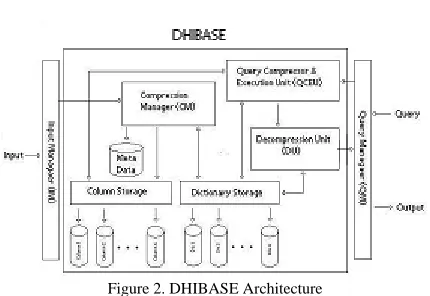
C. DHIBASE: Disk Based HIBASE Model

The basic HIBASE architecture is memory based. We have developed the more general architecture (Fig. 2) that supports both memory and disk based operations. We have made two assumptions:

a. The architecture stores relational database only, b. Single processor database system.

Figure 2. DHIBASE Architecture

The Input Manager (IM) takes input from different sources and passes to Compression Manager (CM). CM compresses the input, make necessary update to appropriate dictionaries and stores the compressed data into respective column storage.

Query Manager (QM) takes user query and passes to Query Compression & Execution Unit (QCEU). QCEU translates the query into compressed form and then apply it against compressed data. Then it passes the compressed result to Decompression Unit (DU) that converts the result into uncompressed form.

(4)

replacing the desired record with the last record and then reducing no of records by one. Dictionary entries are not deleted.

D. DHIBASE: Storage Complexity

SCi = n * Ci bits; where

SCi = space needed to store column i in compressed form

n = no. of records in the relation

Ci = no. of bits needed to represent ith attribute in

compressed form

= ⎡ lg(m) ⎤ , m is no of entries in the corresponding domain dictionary

Total space to store all compressed columns,

bytes, no of column is p

∑

= = p i ci cc S S 1

If we assume that domain dictionaries will occupy 25% of SCC, then Total space to store the compressed relation,

SCR = 1.25 SCC

Total space to store the uncompressed relation,

bits, is the size (in bytes) of

attribute i in uncompressed form.

∑

= × × = p i i UR n x S

1

8 xi

Compression factor, c x c n p x n p S S CF CR UR 25 . 1 8 25 . 1 ) 8 ( ₌ × × × × × × × =

= , assuming that all

attributes have equal width in both compressed and uncompressed form.

IV. DHIBASE: INSERTION, DELETION AND UPDATE

Insertion of a value into a field of record needs the search for compressed code of the given lexeme in the dictionary. If the lexeme is not in the dictionary then we have to add that lexeme to the dictionary which may require widening of the compressed column. Using hash structure, the search requires 2 seeks and 2 blocks transfers. As the last block of the dictionary is in memory, the insertion of the lexeme in the dictionary requires no seeks or block transfers. The complexities of widening operation are given bellow.

Let, B1 and B2 memory blocks are allocated to initial compressed column and widened compressed column respectively. Total block transfers are b1 =

⎡ b m n 8 lg

⎤ and b2 = ⎡ b m n 8 ) 1 (lg +

⎤ respectively; n is the

no of tuples in given relation, m is total no of initial entries in corresponding dictionary and we increase width of the field by 1 bit whenever widening is necessary.

Total no of seeks is

2 2 1 1 B b B b ₊ .

Deletion is performed by replacing the desired record with the last record and then reducing no of records by

one. Dictionary entries are not deleted. Deletion from last memory block needs no seeks or no block transfers. Replacing the desired record by last one requires 2 seeks and 2 blocks transfer for each field.

If the new lexeme is not in the dictionary then we have to insert the new lexeme in the dictionary, which requires all operations of insertion as described in section 3.3. Updating of the desired field of the desired record requires 2 seeks and 2 blocks transfer.

V. SORTING OF COMPRESSED TABLE

Compressed relation contains integer codes. These integer codes correspond to string values stored in dictionary. So we can sort a compressed relation according to codes and also according to the actual string values.

A Sorting According To Code Values

Sorting of table according to code values is required for some queries like natural join. As table is stored in column-wise format, an Auxiliary Column (AC) will be used to help the sorting process. AC has so many rows as the number of records in the table. Initially each row of AC will contain its own position in the column. That is, the ith row of AC contains i. We first sort the column that contains the sorting attribute. Let us consider Table I which will be sorted by CustName.

TABLE I.

CustName Street City Status Johan Kalam Anika Beauty North South West South Gazipur Dhaka Gazipur Gazipur Married Single Married Married

The actual storage (based on dictionaries of Fig. 1) is given in Table II.

TABLE II. CustName 3 2 4 1 Street 2 1 3 1 City 1 2 1 1 Status 1 2 1 1 AC 1 2 3 4

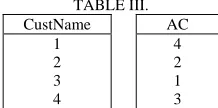
During sorting of CustName column AC will be reordered so that after CustName column is sorted, ith row of AC will contain the initial position of ith row of CustName column. Table III shows CustName and AC columns after sorting of CustName,

TABLE III. CustName 1 2 3 4 AC 4 2 1 3

(5)

ALGORITHM I.

SORTING ACCORDING TO CODE VALUES

Sub SortByCode(byte t, byte c) //sorts tth_{table by its c}th_column

n = no of records in table t

Read all disk blocks of column c of table t into Data() For each record no i of table t , set AC(i) = i call ShellSortCode(Data, AC, n)

Write all blocks in Data() to disk

For each column c1 other than c, call SortCol(Data, AC, c1, n) Delete Data( ), AC( )

End Sub

Sub SortCol(Data(), AC(), c, n)

Read all disk blocks of column c in Data( )

For each entry t in AC(), Write the tth_{compressed record stored in}

Data() to ith_{location of D( )}

Write all blocks of D( ) to disk End Sub

Sub ShellSortCode(Data(), AC(), n)

sorts all of n compressed records stored in Data( ), whenever ith_and

kth_{compressed records are interchanged, the same record no’s of}

AC( ) are also interchanged. End Sub

Let, the column containing the sorting attribute has B disk blocks and M memory blocks are available for sorting disk data. Using external merge sort total no of block transfers to sort the column is B * (2 ⎡logM-1(B/M)⎤

+ 1 ) and total no seeks is 2 * ⎡B/M⎤ + ⎡B/M⎤ (2 * log M-1(B/M)- 1). No of disk blocks to store the Auxiliary

Column (AC) is ⎡ b

n n

8 lg _⎤

; n = no of records and b =

block size in bytes.

B. Sorting According To String Values

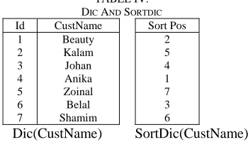
The procedure for sorting a table according to string values is similar to that of sorting according to code values. The only difference is in the method of comparison of two values. Sorting by codes requires comparing only code values stored in the table and needs not checking the corresponding dictionary entries. But sorting by string sorts the table according to dictionary entries of the corresponding code values. This forces to look up strings in the dictionary and then compare those strings. If the strings are very long, the comparison time will be considerably long. To reduce the comparison time we create a dictionary (we call this SortDic, shown in Table IV) for each string domain that stores the sorting position of each code value of the dictionary.

TABLE IV. DIC AND SORTDIC

Id CustName 1

2 3 4 5 6 7

Beauty Kalam Johan Anika Zoinal Belal Shamim

Dic(CustName)

Sort Pos 2 5 4 1 7 3 6

SortDic(CustName) Let us consider the entries 101 (Zoinal) and 111 (Shamim) in CustName column. According to the SortDic(CustName), SortDic(101) = 7 and SortDic(111) = 6. Therefore, ‘111(shamim)’ < ‘101(Zoinal)’. So with SortDic we can avoid long string comparison and thus have faster sorting process. Of course, we have additional space to store SortDic. SortDic only contains integer

values. So they themselves may be stored in compressed form. Hence a particular SortDic consumes a small amount of space and it may be completely kept into main memory to avoid disk access. Also SortDic may be created offline to reduce processing time. Algorithm II describes the technique of sorting by string.

ALGORITHM II.

SORTING ACCORDING TO STRING VALUES

Sub SortByString(byte t, byte c) //sorts tth_{table by its c}th_column

n = no of records in table t

Read all disk blocks of column c of table t into Data() For each record no i of table t , set AC(i) = i call ShellSortString(Data, AC, n)

Write all blocks in Data() to disk

For each column c1 other than c, call SortCol(Data, AC, c1, n) Delete Data( ), AC( )

End Sub

Sub ShellSortString(Data(), AC(), n)

same as ShellSortCode(); but instead of comparing ith_{and k}th

compressed records in Data(), uth_{and v}th_{entries of corresponding}

SortDic are compared. Here u and v are integer values of ith_{and k}th

entries in Data() End Sub

The SortDic is also stored in compressed form. If the domain dictionary has m entries then the no of disk

blocks to store SortDic, N = ⎡ b

m m

8 lg _⎤

; b = block size in

bytes. If we assume that we have N memory blocks to store the entire SortDic then all estimates are same as in Algorithm I.

VI. JOINING IN COMPRESSED FORM

In DHIBASE architecture, columns of same domain share the same single dictionary. Therefore, the same data has same compressed code in all positions in all tables. So we can join two tables based on compressed codes without checking the exact ‘string’ values. Algorithm III describes the natural join of two tables.

ALGORITHM III.

NATURAL JOIN OF T1 AND T2 BASED ON ATTRIBUTE A Sub NaturalJoin(T1, C1, T2, C2) //T2 has total records less than that

//of T1. T1 has column C1 and T2 has column C2 for attribute A Sort T1 according to code values of column C1

Sort T2 according to code values of column C2 Read all disk blocks of column C1 of T1 into D1() Read all disk blocks of column C2 of T2 into D2() Set 1 to both m and j

For each record no k of table T1

While kth_{entry of D1() = j}th_{entry of D2() And}

j <= NoOfRecords(T2) Set kth_{entry of D1() to m}th_{position of D()}

Set k to mth_{position of AC1()}

Set j to mth position of AC2() Increment m and j

Write all blocks of D() to disk For each column k of T1 other than C1

Call Adjust(T1, k, AC1, D1()) For each column k of T2 other than C2,

Call Adjust(T2, k, AC2, D2()) Delete D(), D1(), D2(), AC1(), AC2() End Sub

Sub Adjust(T, C, AC(), Data())

Read all disk blocks of column C of T into Data() For each kth_{entry t of AC()}

set tth_{entry of Data() to k}th_{position of D()}

(6)

We assume that relations T1 and T2 are already sorted. T1 has B1 disk blocks and has n1 tuples and the

no’s for T2 are B2 and n2 respectively. M1 and M2 no of

memory blocks are allocated to store disk blocks of T1 and T2 respectively. Total no of disk block transfers is B1

+ B2. If, on average, p1 tuples of T1 are matched to p2

tuples of T2 then total disk seeks is 2 * max( ⎡n1 / p1⎤ , ⎡n2

/ p2⎤ ) . No of disk blocks to store AC1( ) and AC2( ) are

⎡ b

n n

8 lg ₁

1 _⎤

and ⎡ b

n n

8 lg ₂

2 _⎤

respectively where b is block

size in bytes.

VII. SQL QUERIES ON COMPRESSED DATA

DIHIBASE executes queries directly on compressed data. Following sub-sections describe processing techniques for different types of queries.

A. Queries on Single Table

A.1. Projection

Select C From T. The algorithm is given below:

Read all disk blocks of Dic(C) into D() For each disk block b of column c

For each record r in b Print rth_{entry of D()}

Delete D()

no of seek = 1. no of disk block read = ⎡ b

m n

8 lg

⎤,

here n = no of records and m = no of entries in the domain dictionary.

A.2. Selection with Single Predicate

Select C From T Where Cj = ‘xx’. The algorithm is given

below:

Part-1:

v = code for ‘xx’ in domain Dic(Cj)

Set i = 1

For each disk block b of column Cj

For each record r = v in block b Set r to ith_{position of AC()}

Increment i

Part-2:

Read all disk blocks of Dic(C) into D( )

For each each entry t in AC(), Print tth_{entry of D()}

Using hash structure to search domain dictionary we can find the code for a given ‘string’ in 2 disk seeks and 2 disk-block reads. To select tuples of selection column we

need 1 disk seek and ⎡ b

m n

8 lg

⎤ blocks transfer. The same

no is needed for each projected column. No of disk

blocks to store AC( ) is ⎡ b

n n

8 lg

⎤.

A.3. Selection with Multiple Predicates

Select C From T Where Cj = ‘xx’ And Ck = ‘yy’. The

algorithm is given below:

Part-1 of algorithm given in section VII.A.2 u = code for ‘yy’ in domain Dic(Ck)

For each entry t of AC() If tth_{record of column C}

k is not u, remove t from AC()

Part-2 of algorithm given in section VII.A.2

Selection with q predicates: to search code in domain dictionaries we need q * 1 disk seeks and q * 2 blocks read. To create AC( ) another q * 1 seeks and q *

⎡ b

m n

8 lg

⎤ blocks read are needed. AC() needs ⎡ b

n n

8 lg

⎤

blocks for storage.

A.4 Selection with Range Predicate

Select C From T Where C >= ‘xx’ And C <= ‘yy’. The algorithm is given below:

Let, k and j are the codes for ‘xx’ and ‘yy’ in Dic(C) respectively Let, t1 and t2 are kth_{and j}th_{entries of SortDic(C) respectively}

Now execute the query:

Select C From T Where SortDic(C)>= t1 And SortDic(C)<= t2 SortDic(C) is stored in compressed from. We assume that the total SortDic(C) is in memory which consumes

⎡ b

m m

8 lg

⎤ memory blocks where m is the no of entries in

Dic(C). In worst case when the edge values of the given range are not in Dic(C), we have to search the entire dictionary which requires 1 seek and D blocks transfer ( Dic(C) has D blocks). The modified query further needs 1

seek and a total of ⎡ b

m n

8 lg

⎤ blocks transfer where n is

the total no of records in table T. B. Queries on Multiple Tables

B.1. Projection

Select T1.C From T1, T2. The algorithm is given below:

T = NaturalJoin(T1, T2) Select C’ From T

B.2. Selection with Single Predicate

Select T1.C From T1, T2 Where T1.Cj = ‘xx’. The

algorithm is given below:

T = NaturalJoin(T1, T2)

Select C’ From T Where C’j = ‘xx’

B.3. Selection with Multiple Predicates

Select T1.C From T1, T2 Where T1.Cj = ‘xx’ And T2.Ck =

‘yy’. The algorithm is given below:

T = NaturalJoin(T1, T2)

Select C’ From T Where C’j = ‘xx’ And C’K = ‘yy’

B.4. Set Union

(Select C1 From T1) Union (Select C2 From T2). The algorithm is given below:

Read all disk blocks of C1 of T1 into D1(), Read all disk blocks of C2 of T2 into D2()

Output will be stored into D()

While both D1() and D2() have more elements t = next value from D1()

(7)

move to next value of D1() counter = 0

While D2() has more values and t = next value of D2() move to next value of D2() and increment counter If counter ≠ 0 then insert t into D()

If D1() is finished then

Insert distinct values remaining in D2() into D() Else

Insert distinct values remaining in D1() into D() Endif

Write all blocks of D() to disk

Let, B1, B2 and B memory blocks are allocated to C1, C2 and output column respectively. Total block

transfers are b1 = ⎡ b

m n

8 lg

1 _⎤

, b2 = ⎡ b

m n

8 lg

2 _⎤

and b =

⎡ b

m n

8 lg

⎤ respectively. n1, n2 and n are the no of tuples in

T1, T2 and output respectively, and m is total no of entries in corresponding dictionary. Total no of seeks is

B b B b B

b ₊ ₊

2 2 1 1

.

B.5. Set Intersection

(Select C1 From T1) Intersec (Select C2 From T2). The algorithm is given below:

while D1() has more values and t = next value of D1() move to next value of D1()

counter = 0

While D2() has more values and t = next value of D2() move to next value of D2() and increment counter If counter ≠ 0 then insert t into D()

Write all blocks of D() to disk

Complexities are same that shown in section VII.B.4 (Set Union).

B.6. Set Difference

(Select C1 From T1) Except (Select C2 From T2). The algorithm is given below:

while D1() has more values and t = next value of D1() move to next value of D1()

counter = 0

While D2() has more values and t = next value of D2() move to next value of D2() and increment counter If counter = 0 then insert t into D()

If D1() is not finished then

insert distinct values remaining in D1( )into D( ) Write all blocks of D() to disk

Complexities are same that shown in section VII.B.4 (Set Union).

C. Aggregation

For aggregation queries we shall consider the follow relation:

account(account_no, branch_name, balance)

C.1. Count

select branch_name, count(branch_name) from account group by branch_name. The algorithm is given below: Sort account by branch_name

Read all disk blocks of branch_name column into D() Part-1:

Set c = 1

For each record k in D()

If recent k is different than previous k then Set D1(i) = previous k

Set D2(i) = total no of records having same value as previous k Set c = 1

Part-2:

Write all blocks of D1() and D2() to disk

If M blocks are allocated to each of D( ), D1( ) and

D2( ) then no of block transfer is ⎡ b

m n

8 lg

⎤ for D( ) and

⎡ b

m n n

8 lg ) / (

⎤ for each of D1( ) and D2( ). No of seeks is

3 * ⎡ b

m M

8 lg

⎤. Where n is the average size of each

group.

C.2. Max/ Min

select branch_name, max(balace) from account group by branch_name. The algorithm is given below:

Sort account by branch_name

Read all disk blocks of branch_name column into D() Part-1:

Part-1 of algorithm given in section VII.C.1 Read all disk blocks of column balance into D() base = 0

For each record i of D2()

max = maximum of (base+1)th_{to (base+i)}th_{element of D()}

set D2(i) = max Increment base by i

Complexities are double that shown in section VII.C.1 (Count).

C.3. Sum/ Avg

select branch_name, sum(balace) from account group by branch_name. The algorithm is given below:

Sort account by branch_name

Read all disk blocks of column branch_name into D() Part-1 of algorithm given in section VII.C.1 Read all disk blocks of column balance into D() base = 0

For each record i of D2()

max = sum of (base+1)th_{to (base+i)}th_{element of D()}

// in case of avg make average of these elements set D2(i) = max

Increment base by i

Complexities are same that shown in section VII.C.2 (Max/ Min).

VIII. EXPERIMENTAL RESULTS

(8)

Sales (details are given in the tables bellow). A random data generator has been used to generate synthetic data.

TABLE IV. ITEM RELATIONAL STRUCTRE Attribute

Name

Cardinality Uncompressed field length

(byte)

Compressed field length

(bit) Item_id

(Primary key)

1000 8 10

Type 7 6 3

Description 100 20 7

Total 34 bytes 20 bits (CF = 13.6) TABLE V.

EMPLOYEE RELATION STRUCTURE

Attribute Name

(byte)

(bit) Employee_id

(Primary key)

2000 10 11

Name 400 20 9

Department 15 8 4

Total 38 bytes 24 bits (CF = 12.67) TABLE VI.

STORE RELATION STRUCTURE

Attribute Name

(byte)

(bit) Store_id

(Primary key)

100 6 7

Location 10 10 4

Type 6 6 3

Total 22 bytes _{(CF = 12.57)}14 bits

TABLE VII.

CUSTOMER RELATION STRUCTURE

Attribute Name

(byte)

(bit) Customer_id

(Primary key)

10000 10 14

Name 2000 20 11

City 30 12 5

District 14 12 4

Total 54 bytes 34 bits (CF = 12.71) TABLE VIII.

SALES RELATION STRUCTURE

Attribute Name

(byte)

(bit) Sales_id

(Primary key)

Upto 1 million

(Numeric) 4

32 (Uncompressed) Employee_id

(Foreign key) 2000 10 11

Customer_id

Item_id

Store_id

Quantity Numeric 2 16

(Uncompressed)

Price Numeric 4 32

(Uncompressed)

Total 44 bytes 122 bits (CF = 2.89)

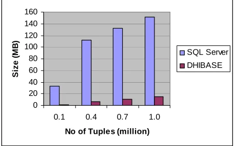
A. Storage Requirement

We have compared our system with widely used SQL Server DBMS. Fig. 3 shows the comparison between DHIBASE and SQL Server storage requirements. We observe that the proposed system outperforms SQL Server by a factor of 10 to 20.

0 20 40 60 80 100 120 140 160

0.1 0.4 0.7 1.0

No of Tuples (million)

Siz

e

(

M

B

)

SQL Server

DHIBASE

Figure 3. Storage comparison between DHIBASE and SQL Server

B. Sorting Of Relation

Fig. 4 shows sorting time needed to sort Sales relation with 0.1, 0.4, 0.7 and 1.0 million records. When we sort a relation based on dictionary code we do not need to refer to the dictionary during sorting. But when we sort a relation based on string order we have to refer to the dictionary. But we avoid this dictionary access by using SortDic( ). The technique is described in section V.B in details. As the SortDic( ) is also compressed and requires small amount of memory, it can be kept into memory during sorting. So the time shown in Fig. 4 indicates that the time needed for sorting based on dictionary code and the time needed for sorting based on string order are same.

C. Query Execution Speed

All queries executed in DHIBASE system are directly applied on compressed data. Given query is first converted into compressed form and compressed query is executed.

C.1. Single Column Projection

We have executed the following query and the result is shown in Fig. 5.

select Customer_id from Sales

0 0.1 0.2 0.3 0.4 0.5 0.6

0.1 0.4 0.7 1

No of tuples (million)

T

im

e

(

m

in

)

(9)

DHIBASE stores data in compressed form and in column wise format. Therefore, it needs 14-bit data to process one record. But SQL Server stores data in row wise format and it needs 44-byte data to process one record. So, in case of 0.1 million records, DHIBASE examines 43 disk blocks (block size = 4K) where SQL Server has to examine 1073 disk blocks. This is the main reason of speed-gain in DHIBASE system.

0 5 10 15 20 25 30 35 40

0.1 0.4 0.7 1.0

T

im

e

(sec

)

SQL Server

DHIBASE

Figure 5. Single column projection

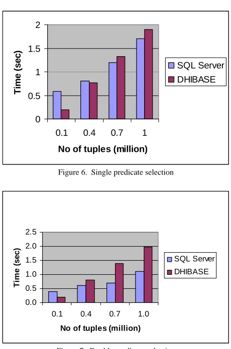
C.2. Single Predicate Selection

select Customer_id from Sales where Store_id = “100075”

Fig. 6 shows that DHIBASE is faster than SQL Server in case 0.1 million to 0.4 million records but slower in case 0.7 million and 1.0 million records. DHIBASE does not use any indices. In case of 1 million records, it reads all 214 disk blocks to check the Store_id column for making a list of desired row no’s. If 100 records satisfy the selection predicate and each of them resides in different disk block then another 100 disk blocks read is necessary to project the Customer_id’s. But SQL Server uses index on Store_id field. So it reads 1 disk block to find pointers to disk blocks containing each of 100 desired records, and needs another 100 disk blocks to read the desired records. So total no of disk block read in SQL Server is 101, which was 314 in DHIBASE.

C.3. Double Predicate Selection

select Customer_id from Sales where Store_id = ‘100075’ and Item_id = “10000300”

Fig. 7 shows result similar to the result of single predicate selection. DHIBASE does not use any indices. In case of 1 million records, it reads all 214 disk blocks to check the Store_id column for making an intermediate list of desired row no’s. If 100 records satisfy the first predicate and each of them resides in different disk block then another 100 disk blocks read is necessary to check the Item_id column for making the final list of desired row no’s. If 10 records satisfy the second predicate and each of them resides in different disk block then another

0 0.5 1 1.5 2

0.1 0.4 0.7 1

Ti

m

e

(

s

e

c

)

SQL Server DHIBASE

Figure 6. Single predicate selection

0.0 0.5 1.0 1.5 2.0 2.5

0.1 0.4 0.7 1.0

T

im

e

(sec

)

SQL Server

DHIBASE

Figure 7. Double predicate selection

10 disk blocks read is necessary to project the Customer_id’s. But SQL Server uses indices on Store_id and Item_id fields. So it reads 1 disk block to find pointers to disk blocks containing each of 100 desired records containing Store_id, also reads 1 disk block to find pointers to disk blocks containing each of 10 desired records containing Item_id and needs another 10 disk blocks to read the desired records. So total no of disk blocks read in SQL Server is 12, which was 324 in DHIBASE. 12 disk blocks read in SQL Server is theoretically minimum. But the actual index structure is not known. And SQL Server uses storage optimization Therefore, the actual no is higher than 12.

C.4. Range predicate selection

select Customer_id from Sales where Store_id >= “100091” and Store_id <= “100100”

(10)

necessary to project the Customer_id’s. But SQL Server, in worst case, may require all 1075 disk blocks to process the scattered Customer_id’s.

0 2 4 6 8 10 12

0.1 0.4 0.7 1

T

ime (

sec) SQL Server

DHIBASE

Figure 8. Selection with range predicate

C.5. Natural Join

select Sales_id from Sales, Customer where Sales.Customer_id = Customer.Customer_id

DHIBASE performs much better because it is possible to calculate the partial join and project the result. DHIBASE does not use any indices. We assume that the relations Sales and Customer are already sorted by Customer_id field according to dictionary code. We have to scan Customer_id columns of both relations to make AC( )’s (section 3.8). In case of 0.1 million records, DHIBASE reads 5 disk blocks to check Customer_id field of Customer relation and 43 disk blocks to check Customer_id field of Sales relation. If the result is scattered across all disk blocks then another 98 disk blocks read is necessary to project Sales_id field of Sales relation. But SQL Server needs to read 134 disk blocks of Customer relation and 1075 disk blocks of Sales relation to compute the join. So SQL Server reads a total of 1209 disk blocks read while DHIBASE read only 141 disk blocks. This is why DHIBASE is much faster. C.6. Aggregation: Count

select Store_id, count (Store_id) from Sales group by Store_id

DHIBASE does not use any indices. We assume that the relation Sales is already sorted by Store_id field according to dictionary code. In case of 0.1 million records, DHIBASE reads all 22 disk blocks of Store_id column to calculate the result. SQL Server uses indices

0 5 10 15 20 25 30 35 40 45

0.1 0.4 0.7 1.0

T

im

e

(sec) SQL Server

DHIBASE

Figure 9. Natural join

0 0.5 1 1.5 2 2.5 3

0.1 0.4 0.7 1.0

T

im

e

(sec

)

SQL Server

DHIBASE

Figure 10. Aggregation: Count

but still it has to read all 1075 disk blocks to process the entire Sales relation. Therefore, DHIBASE performs better than SQL Server.

C.7. Aggregation: Max/ Min/ Sum/ Avg

We have executed the following queries and the result is shown in Fig. 11.

select Store_id, max (Quantity) from Sales group by Store_id

select Store_id, sum (Price) from Sales group by Store_id select Store_id, avg (Price) from Sales group by Store_id

(11)

0 0.5 1 1.5 2 2.5 3 3.5 4

0.1 0.4 0.7 1.0

T

im

e

(sec) SQL Server

DHIBASE

Figure 11. Aggregation: Max/Min/Sum/Avg

C.8. Set Union

(select Customer_id from Customer) union (select Customer_id from Sales)

DHIBASE performs better because it is possible to calculate the result only by scanning Customer_id fields of Customer and Sales relations. DHIBASE does not use any indices. We assume that the Customer_id fields of relations Sales and Customer are already sorted according to dictionary code. DHIBASE reads 5 disk blocks and 43 disk blocks for the relations. But SQL Server reads minimum 134 disk blocks and 1075 disk blocks respectively. So SQL Server reads a minimum of 1209 disk blocks read while DHIBASE read only 48 disk blocks. This is why DHIBASE is much faster.

C.9. Set Intersection/ Set Difference

We have executed the following queries on DHIBASE.

(select Customer_id from Customer) intersect (select Customer_id from Sales)

(select Customer_id from Customer) except (select Customer_id from Sales)

But SQL Server does not support intersection and minus operator directly. So we have executed the following queries on SQL Server.

select distinct Customer_id from Customer where Customer_id in (select Customer_id from Sales)

select distinct Customer_id from Customer where Customer_id not in (select Customer_id from Sales)

In the worst case, both DHIBASE and SQL Server have to examine the entire Customer_id columns of relations of Customer and Sales for both queries, and therefore, time requirements will be similar. Time requirements are shown in Fig. 13.

0 0.5 1 1.5 2 2.5 3

0.1 0.4 0.7 1

T

ime (

s

ec)

SQL Server DHIBASE

Figure 12. Set union

0 0.5 1 1.5 2 2.5

0.1 0.4 0.7 1

Tim

e

(

s

e

c

)

SQL Server DHIBASE

Figure 13. Set intersection/ set difference

DHIBASE performs much better because it is possible to calculate the result only by scanning Customer_id fields of Customer and Sales relations. DHIBASE does not use any indices. We assume that the Customer_id fields of relations Sales and Customer are already sorted according to dictionary code. DHIBASE reads 5 disk blocks and 43 disk blocks for the relations. But SQL Server reads 134 disk blocks and 1075 disk blocks respectively. So SQL Server reads a total of 1209 disk blocks read while DHIBASE read only 48 disk blocks. This is why DHIBASE is much faster. It is mentionable that the result size of four different data sets is same. In case of intersection, DHIBASE reads the smaller relation first. As soon as, this smaller relation finished scanning DHIBASE stops and thus saves time necessary to scan the rest of the other relation.

IX. CONCLUSIONS

(12)

performance SQL queries on single or multiple tables in compressed form.

We have designed and implemented all basic relational algebra operations e.g. selection, projection, join operation, set operations, aggregation, insertion, deletion and update on the architecture. DHIBASE performs better than SQL Server for all operators except selection operation. For projection queries, it is 18 to 22 times faster. This improvement is due to column-wise compressed representation, processing of data in compressed form and less amount of data transfer to and from disk. Selection query is slightly slower than that in SQL Server. This is because DHIBASE architecture does not use any indices. However, this problem may be eliminated by using indices. The architecture can be implemented as a parallel system and a linear scale up is possible in query performance.

REFERENCES

[1] C. B. Tashenberg, “Data management isn’t what it was”, Data Management Direct Newsletter, May 24, 2002. [2] R. Ramakrishnan, J. Goldstein and U. Shaft, “Compressing

relations and indexes”, Proceedings of the IEEE Conference on Data Engineering, pp 370–379, Orlando, Florida, USA, February 1998.

[3] J. T. P. Pucheral and P. Valduriez, “Efficient main memory data management using dbgraph storage”, Prodeedings of the 16th Very Large Database Conference, pp 683 – 695, Brisbane, Queensland, Australia, 1990.

[4] J. S. Karlsson and M. L. Kersten, “W-storage: A self organizing multiattribute storage technique for very large main memories”, Proceedings of Australian Database Conference, IEEE, 1998.

[5] A. Cannane and H. E. Williams, “A compression scheme for large databases”, Proceedings of Australian Database Conference, University of Western Australia, Curtin University, Murdoch University and Edith Cowan University, Perth, 1998, Springer.

[6] N. Kotsis, J. Wilson, W. P. Cockshott and D. McGregor, “Data compression in database systems”, Proceedings of the IDEAS, pp 1–10, July 1998.

[7] D. McGregor, W. P. Cockshott and J. Wilson, “High-performance operations using a compressed architecture”, The Computer Journal, Vol-41, No. 5, pp 283–296, 1998. [8] J. Wilson A. S. M. L. Hoque and D. R. McGregor,

“Database compression using an off-line dictionary method”, ADVIS, LNCS, 2457:11–20, October 2002. [9] D. R. McGregor and A. S. M. L. Hoque, “Improved

compressed data representation for computational

intelligence systems”, UKCI-01, Edinburgh, UK, September 2001.

[10] M. A. Rouf, “Scalable storage in compressed representation for terabyte data management”, M. Sc. Thesis, Department of Computer Science and Engineering, Bangladesh University of Engineering and Technology, Dhaka, Bangladesh, 2006.

[11] D. A. Huffman, “A method for the construction of minimum-redundancy code”, Proceedings of IRE, 40:9:1098–1101, 1952.

[12] A. Lampel and J. Ziv, “A universal algorithm for sequential data compression”, IEEE Transaction on Information Theory, Vol-23, pp 337 – 343, 1977.

[13] A. Lampel and J. Ziv, “Compression of individual sequences via variable rate coding”,IEEE Transaction on Information Theory, Vol-24, pp 530 – 536, 1978.

[14] T.A Welch, “A technique for high-performance data compression”, IEEE Computer, Vol-17, No. 6, pp 8–19, 1984.

[15] G. V., Cormack, “Data compression on a database system”, Communication of the ACM, Vol-28, No. 12, pp 1336–1342, 1985.

[16] S., Helmer, T. D. Westmann, Kossmann and G. Moerkotte, “The implementation and performance of compressed databases”, SIGMOD Record, Vol-29, No. 3, pp 55–67, 2000.

[17] A. Moffat and J. Zobel, “Parameterised compression for sparse bitmap”, Proceedings of the 15th Annual International SIGIR 92, pages 274– 285. ACM, 1992. [18] S. W. Golomb, “Run-length encodings”,IEEE Transaction

on Information Theory, Vol-12, No. 3, pp 399-401, 1966. [19] M. A. Roth, and S. J. Van Horn, “Database compression”,

SIGMOD Record, Vol-22, No. 3, pp 31–39, 1993.

[20] G. Graefe, and L. Shapiro, , “Data compression and database performance”, ACM/IEEE-CS Symposium on Applied Computing, pp 22-27, April 1991.

[21] Oracle Corporation, “Table compression in Oracle 9i: a performance analysis, an Oracle whitepaper”, http://otn.oracle.com/products/bi/pdf/o9ir2_compression_p erformance_twp.pdf.

[22] M. Poess and D. Potapov, “Data compression in Oracle”, Proceedings of the 29th VLDB Conference, pp 937-947, Berlin, Germany, September 2003.

[23] A. Silberschatz, H. F. Korth and S. Sudarshan, “Database system concepts”, 5th Edition, McGraw-Hill, 2006. [24] A. S. M. Latiful Hoque, “Compression of structured and

semi-structured information”, Ph. D. Thesis, Department of Computer and Information Science, University of Strathclyde, Glasgow, UK, 2003.