Robust Facial Features Localization on Rotation
Arbitrary Multi-View Face in Complex
Background
Youjia Fu
College of Optoelectronic Engineering, Chongqing University, Chongqing, 400030 China
College of Computer Science & Engineering, Chongqing University of Technology, Chongqing 400054, China [email protected]
He Yan1 Jianwei Li2, and Ruxi Xiang2
1. College of Computer Science & Engineering, Chongqing University of Technology, Chongqing 400054, China 2. College of Optoelectronic Engineering, Chongqing University, Chongqing, 400030 China
Abstract—Focused on facial features localization on multi-view face arbitrarily rotated in plane, a novel detection algorithm based improved SVM is proposed. First, the face is located by the rotation invariant multi-view (RIMV) face detector and its pose in plane is corrected by rotation. After the searching ranges of the facial features are determined, the crossing detection method which uses the brow-eye and nose-mouth features and the improved SVM detectors trained by large scale multi-view facial features examples is adopted to find the candidate eye, nose and mouth regions,. Based on the fact that the window region with higher value in the SVM discriminant function is relatively closer to the object, and the same object tends to be repeatedly detected by near windows, the candidate eyes, nose and mouth regions are filtered and merged to refine their location on the multi-view face. Experiments show that the algorithm has very good accuracy and robustness to the facial features localization with expression and arbitrary face pose in complex background.
Index Terms—SVM; Facial features localization;
Multi-view facial features localization; Eye detection
I. INTRODUCTION
Face recognition as the front subject of pattern recognition and artificial intelligence has a broad application in the human-machine interface, the biometric information security and so on. The facial features localization is the key of face piece fitting and recognition. Its aim is to determine the face region in the image and locate the eyes, nose, and mouth on it. The past facial features localization algorithms are focused mainly on frontal face, but with the increasing needs for developing actual system, multi-view face recognition has been gradually attached importance and extensive research. However, compared with the frontal facial features localization, the multi-view facial features localization is more complicated, and so its research is relatively weak, more difficult.
At present, the facial features localization methods include the algorithms based on knowledge, such as
integral projection or improved integral projection[1], template matching [2], edge extraction [3] and ASM/AAM [4] etc, which utilize the features of facial grayscale, texture, shape or outline; the algorithms based on statistical learning, such as artificial neural network (ANN), support vector machine (SVM) [5-6] and AdaBoost [7], which regard the facial features as a pattern and extract their common features by statistical learning from lots of examples under different conditions. The former is easy to be influenced by environment, and is also sensitive to the change of face pose. The latter can locate the features well in a variety of complex background and so becomes an effective way to solve the complicated detection problems. Literature [1] realized the fast and accurate eyes localization on multi-view face by projection peak. But because of the integral projection, the algorithm was not suit for the closed eyes. Literature [4] used the improved AAM to locate the feature points accurately, but needed to locate the eyes, nose and mouth at first. Literature [5] presented the two-level SVM algorithm which regarded the linear SVM as the first level and the polynomial SVM as the second one. It achieved 96% of the localization rate of eyes, nose and mouth on the ORL frontal face library. Literature [6] proposed the energy-based framework to jointly perform relevant feature weighting and SVM. It achieved 98% of the eye localization rate on the FERET frontal face library. Literature [7] used the AdaBoost classifier trained by substantial pair of eyes examples to segment the eye regions, and used the fast radial symmetry (FRS) operator to locate the eye centers. It had a very high localization rate on the face with the pose range of [-22.5, 22.5] and got good achievement with [-45, 45]. Because the two eyes need to be both visible in the algorithm, the eye localization on face with larger pose or with rotation both in and off plane was not discussed.
face detector [8], it can realize the features localization on multi-view face with arbitrary rotation in plane. The experiments on the FERET96, the JAFFE, and the database of labeled faces in the wild (LFW) show its robustness and effectiveness in complex environment.
II. IMPROVED SVM LEARNING WITH LARGE SCALE
TRAINING DATA
A. The SVM Theory and Its Limitations
Targeted at the classification problem of two classes, SVM maps the low-dimensional vectors into the high-dimensional space, so that the vectors not separable in the low-dimensional space become as much as possible linearly separable in the high-dimensional one. By constructing an optimal separating surface in the high-dimensional space, SVM achieves the trade-off in ensuring the two classes to have the maximum margin and minimum classification error rate. Given the data set:
D = {(xi, yi)}li=1, xi∈Rd, yi∈{-1, 1}, the SVM problem can be converted into the following quadratic programming problem:
.
.
t
s
l i C y e Q i T T T , ,..., 2 , 1 , 0 0 ) 2 1 min( = ≤ ≤ = + α α α α α, (1)
where T
l)
,..., , (α1α2 α
α= ,αiis the Lagrange multiplier; T
l y y y
y=( 1, 2,..., ) ;
e
is the l-dimensional column vector whose every value is 1; Q is the l×l matrix whose component Qij=yiyjK(xi,xj).Solve the (1) to obtain the classifier
ψ
:∑
= − = l i i iiyK x x b x f 1 ) , ( )
( α , (2)
⎩ ⎨ ⎧ − ≥ = otherwise x f x , 1 ) ( , 1 ) ( θ
ψ , (3)
where f(x) is called the discriminant function of the classifier ψ(x); θ is the adjustment threshold; xi withαi
≠0 is called support vector, obviously, only the support vectors in the (2) are meaningful.
By the (1), we can see that when the number of samples l in the training data set is very large the matrix Q will be also very large, which result in much of memories and very long training time even impossible. So SVM is only very effective on small-scale data set.
B. The Algorithm of Improved SVM
Literature [10] selected a small set randomly from the large sample set for SVM training, and then adjusted the initial set in the whole training samples repeatedly according to KKT conditions until the process converged, so as to solve the problem of SVM learning with large scale training data. Literature [11] pointed out that in the training of incremental SVM, the misclassified samples were often at the boundaries, and were influenced by noise when the sample set was large, but in the case of small scale samples, the misclassified samples reflected the details of the training samples. After the misclassified samples were added to the history training set and trained
again, the support vectors would be closer to the solution. They proved that the accuracy of the classifier would be enhanced with the increment of training samples, so as to approach expectancy risk of the sample space.
By the (2), the optimal separating surface is just determined by the support vectors, and the support vectors can only exist on the boundaries of the two classes. So we select the ones which have the minimum distances in the high-dimensional space according to the (4) in literature [4] as the boundary training samples.
∑
= −= lk
i i kj k kj kj
kj K x x
l x x K d 1
2 ( , ) 2 ( , ) (4)
where K is the kernel function. xkj is the sample j in the class k, and 2
kj
d is the square distance of xkj to the center of the other class. k=1(when k=2)or k=2(when k=1)。 According to the discussion above, our improved SVM training algorithm is as follows, where i is the iteration index:
1) Select the appropriate K, and θ=0, according to the (4) select the m boundary samples from the positive training set A+ and the negative training set A− to form
the work sets (0) + w
A and Aw(0−).
2) Solve the (1) to obtain the support vector sets )
(i sv
A +, Asv(i)− and the classifier ) (i ψ ; 3) Classify A+ and A− by
) (i
ψ , Let (i)
B+ be the
rejected true sample set, (i)
B− be the accepted false
sample set; a) If (i)
B+ ≠Ø, and ) (i
B− ≠Ø, according to the (4)
select n+ samples nearest to B−(i) from B+(i) and n -samples nearest to (i)
B+ from ) (i
B− to form ) (i
N B+
and (i) N B− , let
) ( ) ( ) 1 ( i N i sv i
w A B
A + + + + = + , ) ( ) ( ) 1 ( i N i sv i
w A B
A − − +
− = + ,
go to 2);
b) If (i)
B+ =Ø, B−(i) ≠Ø, according to the (4) select n- samples nearest to Asv(i)+ from B−(i) to form
) (i
N B− , let
) ( ) 1 ( i sv i w A A + + + = , ) ( ) ( ) 1 ( i N i sv i
w A B
A − − +
− = + ,go to 2);
c) If (i)
B+ ≠Ø, B−(i) =Ø, according to the (4)
select n+ samples nearest to Asv(i)− from ) (i B+ to
form (i) N
B+ , let ( 1) () (iN) i sv i
w A B
A++ = ++ + , ( 1) sv(i) i
w A
A−+ = −,go to
2);
d) If (i)
B+ =Ø, and B−(i)=Ø, the training is end
and the last classifier ψ(i)is the one we need. If the number of the samples in (i)
B+ or ) (i
B− is less
than n+ or n-, then let B+(iN) = ) (i
B+ or B−(iN)= ) (i B− .
III. THE ALGORITHM IMPLEMENT OF MULTI-VIEW
FACIAL FEATURES DETECTION
A. The Frame of Multi-View Facial Features Localization
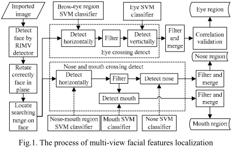
level 1 is for the horizontal windows and the SVM level 2 is for the vertical windows. The horizontal windows contain respectively the brow-eye and the nose-mouth regions which help to distinguish the features from background. The vertical windows focus on the distinctions between the eye and brow, the nose and mouth.
Fig.1. The process of multi-view facial features localization
B. The RIMV Face Detector
The RIMV face detector in the literature [8] adopts the Multi-view face detector (MVFD) which covers a large range of the face pose between +/-45º rotation in plane (RIP), and +/-90º rotation off plane (ROP). By simply rotating the MVFD 90º, 180º and 270º, the RIMV face detector implements the detection of the multi-view face with rotation arbitrary in plane.
C. The Crossing Detection Method
As the eye is only situated on the upper half of face and under the forehead, just this part of region will be searched for eye. Let P(x, y) be the point in the searching region, the hface and wface are the height and width of the face rectangular region. So for the brow-eye region, 0≤x≤wface,11/48hface≤y≤7/12hface; for the nose-mouth region, 1/8wface≤x≤7/8wface,1/2hface≤y≤hface. After the nose-mouth region is determined, the range of 0.5hface≤y≤0.8hface is selected as the vertical nose searching region, and the 0.6hface≤y≤1.2hface as the vertical mouth searching region. The searching regions not only cover the facial features on the multi-view face with RIP of [-20, 20], but also eliminate the hair and other background.
Our crossing searching method contains two types of windows: the horizontal detection window moves horizontally to find the brow-eye and nose-mouth regions; the vertical detection window moves vertically in the horizontal regions to find the eyes, nose and mouth. Let
heye be the height of eye searching region; heh and weh be
the height and width of the horizontal brow-eye detection window, having heh = heye. As the width ratio of eye to
face is about 1/5, so weh = 0.2wface. Let teh be the moving
step of the horizontal window, so teh = 0.25weh. Let hev,
wev and tev be the height, width and move step of the
vertical eye window. The window contains the whole eye, so wev = weh, hev =0.4heh, tev = 0.25hev. After vertical
detection, brow is excluded and the candidate eye region is obtained.
Just like the eyes search, let hnm be the height of
nose-mouth searching region, hnmh and wnmh are the
height and width of the horizontal nose-mouth detection window, then hnmh = hnm, the window width is the same
as the nose, so wnmh = 0.25wface; the move step tnmh =
0.125wnmh. Let hnv, wnv and tnv be the height, width and
move step of the vertical nose detection window, then wnv
= wnmh, hnv = 0.25hnmh, tnv = 0.25hnv. Let hmv, wmv and tmv
be the height, width and move step of the vertical mouth detection one. For the convenience of traversal, the wmv is
slightly less than the mouth, then wmv = wnv = wnmh, hmv =
0.4hnmh and tmv = 0.125 hmv. After vertical detection, the
candidate nose and mouth regions are obtained.
D. The Multi-view Facial Features Samples
From the FERET, we select the images containing the faces with naked eyes,with glasses, and with the poses at 0°, 22.5°, 45°, 67.5° and 90°. Because the error of face RIP detected by RIMV face detector is about between 0° and 20°, we rotate these images ±10° and ±20° respectively and get the total 1400 faces which can be detected by RIMV detector correctly. From them 1450 brow-eye samples and 2400 “non-brow-eye” samples are cut out, and their sizes are normalized to 28×40; 933 nose-mouth samples and 1629 “non-nose-mouth” samples are cut out, and normalized to 28×56. In the same way, 1930 eye samples and 4600 non-eye samples are cut out and normalized to 28×16; 402 nose samples and 4015 non-nose samples are cut out and normalized to 28×14; 504 mouth samples and 3253 non-mouth samples are cut out and normalized to 28×22. Parts of the samples are shown in Fig. 2.
Fig. 2 Parts of facial feature training samples: (a) brow-eye samples, (b) “non-brow-eye” samples, (c) eye samples, (d) non-eye samples, (e) nose-mouth samples, (f) “non-nose-mouth” samples, (g) nose samples,
(h) non-nose samples, (i) mouth samples, (j) non-mouth samples
E. The Implementation of the SVM Training and Detection
We select the quadratic polynomial as the SVM kernel function, and C=1.0. The horizontal window classifier Ψh and the vertical window classifier Ψv are
obtained by the training algorithm in the paragraph B of section II. Because the number of negative samples is much more than the positive ones, the SVM classification result tends to false reject instead of false acceptance, then the θ in the (3) is taken a relatively low value to ensure that the regions detected out contain the true features. By experiment, for the eye θ=-0.18 in Ψh, and
θ=-0.44 in Ψv; for the nose and mouth θ=-1.08 in Ψh,
θ=-0.50 in Ψnose; and θ=-1.70 in Ψmouth.
IV. FILTERING AND MERGING THE DETECTED REGIONS
According to the SVM property, the sample which has higher value in the (2) tends to be farther to the separating surface. In order to make the regions detected out as accurate as possible, we do not regard the outputs of the positive windows Ψas the candidate regions just like the traditional algorithm; instead, process the detection results as the following methods.
A. The Filter and Localization of Eye Regions A.1. Filtering the candidate eye regions
1) Sort the regions traversed by the horizontal window in descending order according to their values in the (2), and obtain the region sequence qh={
h f1 ,
h f2 ,…,
h n
f }. Let SA and SB be the two horizontal regions of
candidate eyes. 2) Select h
f1 into SA. If Ψh=1 for f1h according to the (3), continue to access qh and select the first 3 regions which meet the following conditions into SA.
a) Ψh =1 for the region according to the (3); b) Let nt be the number of the step which the window moves from this region to h
f1 , having 0<| nt | ≤3.
3) Traverse qh and select the first region that does not intersect with SA as SB. Let this region befph. IfΨh =1 for h
p
f according to the (3), select the first 3 regions into
SB by the similar way in the step 2).
4) Traverse vertically the SA and SB, and sort the
detection regions in descending order according their values in the (2). Select the first 3 regions from each SA
and SB whoseΨv =1 according to the (3) as the candidate
eye regions.
A.2. Process the overlapping eye windows
Because the detection step is small, the adjacent window regions have a high similarity. The same eye may be detected by several adjacent windows, which will result in multiple overlapping candidate eye regions. So we process them as follows:
Let seq={R1, R2,…,Rn} be the sequence of the candidate eye regions in each SA and SB, where
Rk=(x,y,w,h) is the rectangle; (x, y) is its coordinate of the upper-left corner, w and h are its width and height. For Rk
and Rt,, let Dw = 0.5×Rt.w, Dh=0.5×Rt.h; if the two rectangles meet the following conditions, they overlap each other: 1) Rk.x<Rt.x+Dw; 2) Rk.x>Rt.x-Dw; 3) Rk.y<Rt.y+Dh; 4) Rk.y>Rt.y-Dh.
After overlapping detection, the overlapping rectangle windows form the group. Let Seqop={g1, g2, …,
gm} be the group sequence in SA or SB. The single
rectangle window is also as a group in the Seqop. Let gi∈
Seqop, n is the number of the rectangle windows in gi, n≥1. { i
f1, i f2,…,
i n
f } are the windows values in the (2) in the
gi, and fi=
∑
= nj i j f n 1
1 . We select the groups which have the
most overlapping windows to form the sequence Seq1,
Seq1
⊆
Seqop, From Seq1 we select the group with maximali
f as the candidate eye group in SA or SB. The average
rectangle of the candidate eye group is regard as the last eye region.
B. The Filter and Localization of Nose and Mouth Regions
1) Sort the horizontal window regions in descending order according their values in the (2) and select the first 8 regions whose Ψh =1 according to the (3) as the
candidate nose-mouth regions.
2) Traverse vertically the nose searching regions in the nose-mouth regions, and sort the detection regions in descending order according their values in the (2). Select the first 8 regions whose Ψnose =1 according to the (3) as
the candidate nose regions.
3) Traverse vertically the mouth searching regions in the nose-mouth regions, and sort the detection regions in the same way. Select the first 12 regions whose Ψmouth =1
according to the (3) as the candidate mouth regions. 4) Determine the overlapping window groups of nose and mouth by the method in the paragraph A.2. Select the groups with the maximal i
f from the ones which have the most overlapping windows as the candidate nose and mouth groups. Their average rectangles are the nose and mouth regions.
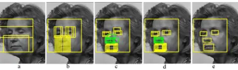
Fig. 3 illustrates the whole process of detecting and filtering the eyes, nose and mouth regions.
Fig.3. A illustration of detecting and filtering the facial features regions: (a) the face and its feature searching regions, (b) the brow-eye and nose-mouth regions, (c) the candidate features regions, (d) the candidate
features region after filtering, (e) the eyes, nose and mouth regions
V. EXPERIMENTS AND EVALUATION
A. Dataset
faces is that they can be detected by the Viola-Jones face detector. All the image size in the LFW is 250×250.
We select randomly the faces which are different from the training samples from FERET. They contains the pose at 0°, 15°, 22.5°, 45°, 67.5° and 90°. Every face is rotated by ±10° first, then rotated once every 20° and 360° of total in plane. After the faces that can not be detected by the RIMV face detector being removed, total 1630 test samples are obtained.
We select randomly 400 images from the LFW, which contain the faces with different pose, expression, wearing glasses, opening or closing eyes, and low clarity.
JAFFE contains ten people, seven expressions, total 213 images. All the images can be detected by Adaboost face detector, and so used for the test.
B. Evaluation Protocol
To evaluate the precision of eye localization, the relative error measurement [7] is used as the localization criterion. Let Cle and Cre be the centers of the automatic located left and right eyes; '
le
C and Cre' are the centers of the manual marked ones; the relative error is defined as:
eye err =
| |
|) |
|, max(|
' '
' '
re le
re re le le
C C
C C C C
− −
− (5)
Let Cnm be the center of the automatic located nose or mouth; '
nm
C is the center of the manual marked ones; the relative error is defined as:
) ( mouth
nose err err =
|) |
|, min(|
| |
' ' ' '
'
re nm le nm
nm nm
C C C C
C C
− −
− (6)
If err<0.20, the localizations are considered as success.
C. Experimental Results and Evaluation
Our test environment is: Intel Core2 3.0GHz CPU, 2G Memory, Windows XP operating system, Matlab 2007, VC.NET 2005 and OpenCV. The multithreaded programming technique is adopted in our system. One thread is used to locate the eyes, and the other parallel thread is used to locate the nose and mouth.
1) The experiments on multi-view faces
The table Ι shows the localization result presented in the literature [7] on the FERET. The tables II-IV show the localization result of our facial features algorithm combined with the Viola-Jones face detector on the FERET. The table V shows our localization result combined with the Vector Boosting detector [8] on the FERET with arbitrary rotation in plane.
The “SA” in the tables means the swing angles that face rotates around the vertical axis, and the “TA” means the tilting angle that face rotates around the normal axis of view plane. From the tables, we can see that our method has the very high accuracy rate under the swing angle range [-22.5°, 22.5°] and the tilting angle range [-10°, 10°], just equivalent to the literature [7] and [1] (97.3% of the eye localization rate on the FERET; 98.78% on the JAFFE). To the face with arbitrary pose, our method also achieves better accuracy rate than literature [7].
Shown from the table II to table V, the localization rate of nose and mouth are significantly higher than the eyes on the multi-view face. On the one hand because the eye features are complex than the nose and mouth; on the other hand when the face pose is large, the farther eye becomes small, which weakens its feature, but the face pose affects the nose and mouth relatively slightly.
TABLEI. RESULTS PRESENTED IN THE LITERATURE [7] ONFERET(ERR<0.2)
Swing Angle -45 -22.5 0 22.5 45
Proportion 79.6 98.1 100 97.4 80.2
TABLEII. OUR EYE LOCALIZATION RESULTS ONFERET(ERR<0.2)
SA
TA 0 ±15 ±22.5 ±45
More than ±67.5 0 100 100 98.0 88.0 82.2
±10 97.4 97.2 94.1 86.2 79.5
±20 93 91.6 84.3 82.7 75.3
TABLE III. OUR NOSE LOCALIZATION RESULTS ON FERET (ERR<0.2)
SA
TA 0 ±15 ±22.5 ±45 More than ±67.5
0 100 100 98.0 98.0 92.0 ±10 99.0 99.0 96.4 92.4 90.5 ±20 98.5 98.0 85.7 91.3 80.9
TABLE IV. OUR MOUTH LOCALIZATION RESULTS ON FERET (ERR<0.2)
SA
TA 0 ±15 ±22.5 ±45 More than ±67.5
0 100 98.0 98.0 100 96.0 ±10 99.0 99.0 99.0 100 96.2 ±20 100 100 98.1 93.5 93.1
TABLE V. OUR AVERAGE LOCALIZATION RATE ON FERET WITH
ARBITRARY ROTATION IN PLANE (ERR<0.2)
Swing
Angle 0 ±15 ±22.5 ±45
More than ±67.5 eye 95.2 95.3 91.3 83.7 80.3 nose 97.8 97.2 91.6 92.7 88.4
mouth 99.1 98.7 97.8 94.3 92.5
2) The robustness experiments
Shown in the table VI and VII, our method has a very strong robustness to the front expression face under err<0.15. To the images with different poses, expressions and low clarity, our method also has a strong robustness under err<0.20. The experiments also demonstrate that the locating speed of our method is about 0.14s for one image with 250×250 size. The parts of experimental results in the test images are shown in Fig.4.
TABLE VI. OUR RESULTS ON JAFFE
Precision err<0.05 err<0.10 err<0.15 err<0.20 err<0.25 eye 22.2 60.9 97.6 98.6 98.6 nose 73.4 95.2 100 100 100 mouth 45.9 94.7 100 100 100
TABLE VII OUR RESULTS ON LFW
Fig.4. Some experimental results on the test images
VI. CONCLUSION
To solve the problem of locating facial features region on the rotation arbitrary multi-view face in complex background, we propose a robust localization method, which use a coarse-to-fine strategy to locate the eyes, nose and mouth regions on the face detected by the face detector. The contributions in the article are as follows: 1) First, the horizontal regions of facial features are found by the brow-eye and nose-mouth features, then the candidate eyes, nose and mouth are obtained along the vertical direction by their respective features, which enhances the facial features and facilitates to distinguish from background. 2) The improved SVM trained by large scale data are used to form the two-level classifier, which enhances the classification accuracy. 3) Based on the fact that the window region with higher value in the SVM discriminant function is relatively closer to the object, and the same object tends to be repeatedly detected by near windows, the candidate facial feature regions are selected conditionally and filtered, which effectively avoid the impact produced by the possible SVM overtraining. The experiments demonstrate that combined with the RIMV face detector our algorithm can effectively locate the facial features with arbitrary pose in complex background.
REFERENCES
[1] DAI Jinwen, LIU Dan, SU Jianbo. “Rapid eye location based on projection peak,” Chinese Journal of Pattern Recognition and Artificial Intelligence, 2009, vol. 22, pp. 605-609. (in Chinese)
[2] WANG Jian, ZHAO Honglian. “Eye detection based on multi-angle template matching,” //Proceedings of 2009 International Conference on Image Analysis and Signal Processing, Linhai, China, 2009, pp. 241-244.
[3] W. M.K Wan Mohd Khairosfaizal, A.J.Nor’aini. “Eyes detection in facial images using circular hough transform,” //Proceeding of 2009 5th International Colloquium on Signal Processing and Its Applications, CSPA 2009, pp. 238-242.
[4] FAN Xiaojiu, Peng Qiang, Jim X Chen, Xia Xu. “An improved AAM fast localization method for human facial
features,” Chinese Journal of Electronics & Information Technology, 2009, vol. 31, pp. 1354-1358. (in Chinese) [5] LI Dihua, Podolak LT, Lee S. W. “Facial component
extraction and face recognition with support vector machines,” //Proceeding of 2002 2th IEEE International Conference on Automatic Face and Gesture Recognition, Washington DC, USA. New York: IEEE Press, 2002, pp. 76-81.
[6] Minh Hoai NGUYEN, Joan PEREZ, Fernando De La TORRE. “Facial feature detection with optimal pixel reduction SVM,” //Proceeding of 2008 8th IEEE International Conference on Automatic Face and Gesture Recognithon. New York: IEEE Press, 2008, pp. 376-381. [7] ZHANG Wencon, LI Xin, YAO Peng, LI Bin, ZHUANG
Zhenquan. “A Robust eye localization algorithm for face recognition,” Chinese Journal of Electronics, 2008, vol. 25, pp. 337-342.
[8] Huang Chang, Ai Haizhou, Li Yuan, Lao Shihong. “Vector Boosting for Rotation Invariant Multi-View Face Detection,” //Proceeding of the Tenth IEEE International Conference on Computer Vision(ICCV’05), Beijing, China. 2005.
[9] http://vis-www.cs.umass.edu/lfw/, 2010, 4.
[10] Osuna E, Freund R, Girosi F. “An improved training algorithm for support vector machine,” //Proceedings of the 1997 IEEE Workshop on Neural Networks for Signal Processing. New York: IEEE Press, 1997, pp. 276-285. [11] XIAO Rong, WANG Jicheng, SUN Zhengxing, ZHANG
Fuyan. “An approach to incremental SVM learning algorithm,” Journal of Nanjing University (Natural Sciences), 2002, vol. 38, pp. 152-157. (in Chinese)
[12] ZHENG Zhixun, YANG Jiangang. “New method of SVM learning with large scale training data,” Chinese Journal Computer Engineering and Design, 2006, vol. 27, pp. 2425-2431. (in Chinese)
Youjia Fu was born in 1974. He is currently a Ph.D.
candidate in college of optoelectronic engineering, Chongqing University, Chongqing, China. He received his B.S degree from Wuhan University of Technology, Wuhan, in 2005. His research interests include pattern recognition, digital image processing, computer graphics and virtual reality.
He Yan was born in 1972. He is currently an associate
professor of computer science, Chongqing University of Technology, Chongqing, China. He received his Ph.D. degree from Chongqing University, Chongqing, China, in 2009. His research interests include digital image processing, artificial intelligence, spatial database.
Jianwei Li was born in 1947. He is currently a professor of
computer science, Chongqing University. His research interests include pattern recognition, digital image processing and GIS.
Ruxi Xiang is currently a Ph.D. candidate in college of