Comparative Analysis of Rate of Convergence of
Agarwal et al., Noor and SP iterative schemes for
Complex Space
Renu Chugh, Vivek Kumar ,Ombir Dahiya
Department of MathematicsMaharshi Dayanand University, Rohtak, India
ABSTRACT
In this paper, we analyze the rate of convergence of three iterative schemes namely-Agarwal et al., Noor and SP iterative schemes for complex space by using Matlab programmes. The results obtained are extensions of some recent results of Rana, Dimri and Tomar[1].
General Terms
Computational Mathematics
Keywords
Agarwal et al. iterative scheme, Noor iterative scheme, SP iterative scheme
1. INTRODUCTION
Although fixed point iterative schemes are used in solving problems of industrial and applied mathematics still there is no systematic study of numerical aspects of these iterative schemes. In computational mathematics, it is important to compare the iterative schemes with regard to their rate of convergence. By using computer programs, perhaps for the first time, B. E. Rhoades [2] illustrated the difference in convergence rate of Mann and Ishikawa iterative procedures for increasing and deceasing functions through examples. S. L. Singh[3] extended the work of Rhoades. In [4,5] Berinde showed that Picard iteration converges faster than Mann iteration for quasi-contractive operators.
Recently, Nawab Hussian et al. [6] provide an example of a quasi-contractive operator for which the iterative scheme due to Agarwal et al. is faster than Mann and Ishikawa iterative schemes. By providing examples, W. Phuengrattana and S. Suantai[7] showed that SP iterative scheme converges faster than Mann, Ishikawa and Noor iterative for nondecreasing and continuous functions on real line intervals. Recently, Rana, Dimri and Tomar[1] showed that Ishikawa iterative scheme converges faster than Mann iterative scheme while Picard iterative scheme converges faster than both in complex space.
2. PRELIMINARIES
Let (X, d) be a complete metric space and T: X
X a selfmap of X. Suppose that F(T) ={ pX, Tp = p} is the set of fixed points of T. There are several iterative processes in the literature for which the fixed points of operators havebeen approximated over the years by various authors. In a complete metric space, the Picard iterative process
xn n0 defined byxn1Txn n = 0, 1,… (2.1)
is used to approximate the fixed points of mappings satisfying the following Banach’s contraction condition: (d Tx Ty, ) d x y( , ) (2.2) for all x , y X and [0, 1).
In 1953, W. R. Mann defined the Mann iteration [8] as
xn1 (1 n)xnnTxn (2.3)
where {n} is a sequences of positive numbers in [0,1]. In 1974, S. Ishikawa defined the Ishikawa iteration [9] as
xn1 (1 n)xnnTyn
yn (1 n)xnnTxn, (2.4) where {n} and {n} are sequences of positive numbers in
[0,1].
In 2007, Agarwal et al. defined the Agarwal et al. iterative scheme [10] as
sn1 (1 n)TsnnTtn tn (1 n)snnTsn, (2.5)
where {n} and {n} are sequences of positive numbers in
[0,1].
In 2000, M. A. Noor defined the three step Noor iteration [11] as
xn1 (1 n)xnnTyn yn (1 n)xnnTzn
zn (1 n)xnnTxn , (2.6) where {n}, {n} and {n} are sequences of positive numbers in [0,1].
Phuengrattana and Suantai defined the SP iteration [7] as
xn1 (1 n)ynnTyn yn (1 n)znnTzn
zn (1 n)xnnTxn , (2.7) where {n}, {n} and {n} are sequences of positive numbers in [0,1].
Remarks
2. If n=n= 0, then Noor iteration (2.6) reduces to the Mann iteration (2.3).
3. If n=n= 0, then SP iteration (2.7) reduces to the Mann iteration (2.3).
In this paper, we take ' ''
n s, n s, n s
and derive the fixed points of the following polynomial functions :
Quadratic functions = z2 + c Cubic functions = z3 + c Biquadratic functions = z4 + c
Recently, Rana, Dimri and Tomar[1] draw a comparative analysis of Picard, Mann and Ishikawa iterative schemes by starting with z = (0,0) and c = 0.1 in complex space.
In this paper, we will continue the comparative study in complex space by taking same z and c, for Agarwal et al., Noor and SP iterative schemes and hence extend the results of Rana, Dimri and Tomar[1] .
3. EXPERIMENTS
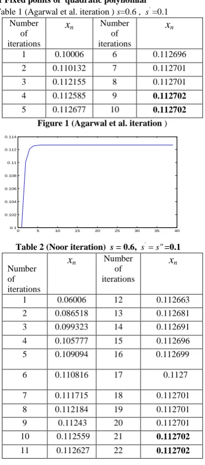
3.1 Fixed points of quadratic polynomial Table 1 (Agarwal et al. iteration ) s=0.6 , '
s=0.1 Number
of iterations
x
n Numberof iterations
x
n1 0.10006 6 0.112696
2 0.110132 7 0.112701
3 0.112155 8 0.112701
4 0.112585 9 0.112702
5 0.112677 10 0.112702
Figure 1 (Agarwal et al. iteration )
0 5 10 15 20 25 30 35 40
0.1 0.102 0.104 0.106 0.108 0.11 0.112 0.114
Table 2 (Noor iteration) s = 0.6, '
" s s =0.1
Number of iterations
x
n Numberof iterations
x
n1 0.06006 12 0.112663
2 0.086518 13 0.112681
3 0.099323 14 0.112691
4 0.105777 15 0.112696
5 0.109094 16 0.112699
6 0.110816 17 0.1127
7 0.111715 18 0.112701
8 0.112184 19 0.112701
9 0.11243 20 0.112701
10 0.112559 21 0.112702
11 0.112627 22 0.112702
Figure 2 ( Noor iteration)
0 5 10 15 20 25 30 35 40 45 50
0.06 0.07 0.08 0.09 0.1 0.11 0.12
Table 3 (SP iteration ) s=0.6, '
" s s =0.1 Number
of iterations
x
n Numberof iterations
x
n1 0.067821 10 0.112667
2 0.093306 11 0.112686
3 0.104064 12 0.112695
4 0.108806 13 0.112698
5 0.110935 14 0.1127
6 0.111899 15 0.112701
7 0.112336 16 0.112701
8 0.112535 17 0.112702
9 0.112626 18 0.112702
Figure 3 (SP iteration)
0 5 10 15 20 25 30 35 40 45 50
0.065 0.07 0.075 0.08 0.085 0.09 0.095 0.1 0.105 0.11 0.115
Table 4 (Agarwal et al. iteration ) s = 0.6 , '
s=0.3 Number
of iterations
x
n Numberof iterations
x
n1 0.10054 6 0.112699
2 0.11046 7 0.112701
3 0.112271 8 0.112702
4 0.112618 9 0.112702
5 0.112685 10 0.112702
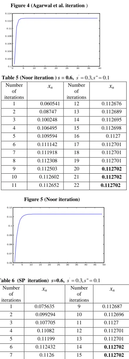
[image:2.595.63.271.290.762.2]Figure 4 (Agarwal et al. iteration )
0 5 10 15 20 25 30 35 40
0.1 0.102 0.104 0.106 0.108 0.11 0.112 0.114
Table5 (Noor iteration ) s = 0.6, s'0.3, "s 0.1 Number
of iterations
x
n Numberof iterations
x
n1 0.060541 12 0.112676
2 0.08747 13 0.112689
3 0.100248 14 0.112695
4 0.106495 15 0.112698
5 0.109594 16 0.1127
6 0.111142 17 0.112701
7 0.111918 18 0.112701
8 0.112308 19 0.112701
9 0.112503 20 0.112702
10 0.112602 21 0.112702
11 0.112652 22 0.112702
Figure 5 (Noor iteration)
0 5 10 15 20 25 30 35 40 45 50
0.06 0.07 0.08 0.09 0.1 0.11 0.12
Table 6 (SP iteration) s=0.6, '
0.3, " 0.1
s s
Number of iterations
x
n Numberof iterations
x
n1 0.075635 9 0.112687
2 0.099294 10 0.112696
3 0.107705 11 0.1127
4 0.11082 12 0.112701
5 0.11199 13 0.112701
6 0.112432 14 0.112702
7 0.1126 15 0.112702
8 0.112663 16 0.112702
Figure 6 ( SP iteration)
0 5 10 15 20 25 30 35 40 45 50
0.075 0.08 0.085 0.09 0.095 0.1 0.105 0.11 0.115
Table 7 (Agarwal et al. iteration ) s = 0.6 , '
s= 0.5 Number
of iterations
xn Number
of iterations
xn
1 0.1015 6 0.1127
2 0.11085 7 0.112701
3 0.112384 8 0.112702
4 0.112647 9 0.112702
5 0.112692 10 0.112702
Figure 7 (Agarwal et al. iteration )
0 5 10 15 20 25 30 35 40
0.1 0.102 0.104 0.106 0.108 0.11 0.112 0.114
Table 8 (Noor iteration ) s=0.6, '
0.5, " 0.4 s s
Number of iterations
x
n Numberof iterations
x
n1 0.061548 12 0.112687
2 0.088838 13 0.112695
3 0.101424 14 0.112698
4 0.107339 15 0.1127
5 0.110145 16 0.112701
6 0.111481 17 0.112701
7 0.112118 18 0.112701
8 0.112423 19 0.112702
9 0.112568 20 0.112702
10 0.112638 21 0.112702
11 0.112671 22 0.112702
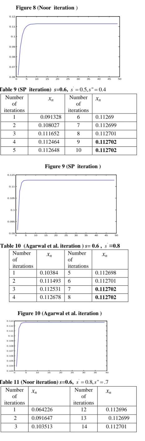
[image:3.595.60.538.67.660.2] [image:3.595.58.278.68.680.2] [image:3.595.317.539.69.694.2]Figure 8 (Noor iteration )
0 5 10 15 20 25 30 35 40 45 50
0.06 0.07 0.08 0.09 0.1 0.11 0.12
Table 9 (SP iteration) s=0.6, '
0.5, " 0.4 s s
Number of iterations
x
n Numberof iterations
x
n1 0.091328 6 0.11269
2 0.108027 7 0.112699
3 0.111652 8 0.112701
4 0.112464 9 0.112702
5 0.112648 10 0.112702
Figure 9 (SP iteration )
0 5 10 15 20 25 30 35 40 45 50
0.09 0.095 0.1 0.105 0.11 0.115
Table 10 (Agarwal et al. iteration ) s= 0.6 , s'
=
0.8 Numberof iterations
x
n Numberof iterations
x
n1 0.10384 5 0.112698 2 0.111493 6 0.112701 3 0.112531 7 0.112702 4 0.112678 8 0.112702
Figure 10 (Agarwal et al. iteration )
0 5 10 15 20 25 30 35 40
0.103 0.104 0.105 0.106 0.107 0.108 0.109 0.11 0.111 0.112 0.113
Table 11 (Noor iteration) s=0.6, '
0.8, " .7
s s
Number of iterations
x
n Numberof iterations
x
n1 0.064226 12 0.112696 2 0.091647 13 0.112699
4 0.108682 15 0.112701 5 0.110942 16 0.112701
6 0.111931 17 0.112702 7 0.112364 18 0.112702 8 0.112554 19 0.112702 9 0.112637 20 0.112702
10 0.112673 21 0.112702
11 0.112689 22 0.112702
Figure 11 (Noor iteration )
0 5 10 15 20 25 30 35 40 45 50
0.06 0.07 0.08 0.09 0.1 0.11 0.12
Table 12 (SP iteration) s = 0.6, '
0.8, " 0.7
s s
Number of iterations
x
n1 0.104921
2 0.111992
3 0.112636
4 0.112696
5 0.112701
6 0.112702
7 0.112702
Figure 12 (SP iteration)
0 5 10 15 20 25 30 35 40 45 50
0.104 0.105 0.106 0.107 0.108 0.109 0.11 0.111 0.112 0.113 0.114
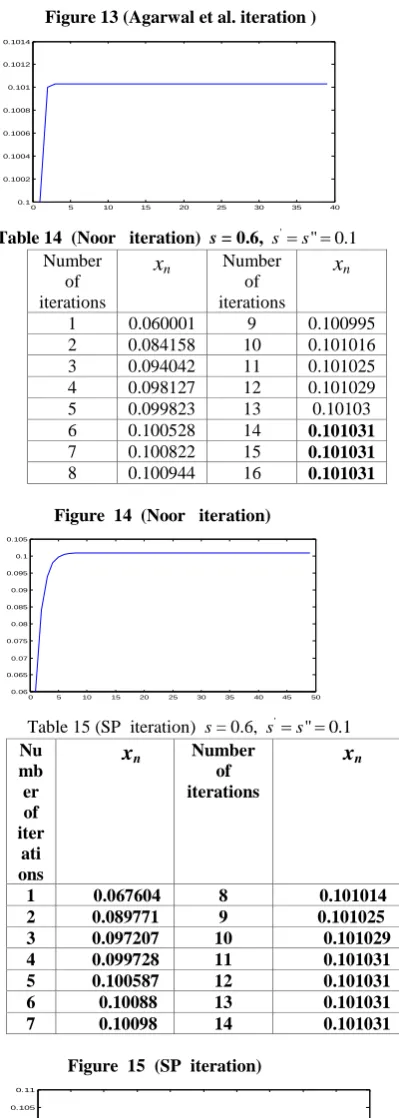
3.2 Fixed points of cubic polynomial Table 13 (Agarwal et al. iteration ) s = 0.6 , '
s
=
0.1
Number of iterationsx
n1 0.100001
2 0.101002
3 0.10103
[image:4.595.59.539.61.768.2] [image:4.595.56.290.65.774.2] [image:4.595.322.537.67.577.2]Figure 13 (Agarwal et al. iteration )
0 5 10 15 20 25 30 35 40
0.1 0.1002 0.1004 0.1006 0.1008 0.101 0.1012 0.1014
Table 14 (Noor iteration) s = 0.6, '
" 0.1 ss Number
of iterations
x
n Numberof iterations
x
n1 0.060001 9 0.100995
2 0.084158 10 0.101016
3 0.094042 11 0.101025
4 0.098127 12 0.101029
5 0.099823 13 0.10103
6 0.100528 14 0.101031
7 0.100822 15 0.101031
8 0.100944 16 0.101031
Figure 14 (Noor iteration)
0 5 10 15 20 25 30 35 40 45 50
0.06 0.065 0.07 0.075 0.08 0.085 0.09 0.095 0.1 0.105
Table 15 (SP iteration) s = 0.6, '
" 0.1
ss
Nu mb er of iter ati ons
x
n Numberof iterations
x
n1 0.067604 8 0.101014
2 0.089771 9 0.101025
3 0.097207 10 0.101029
4 0.099728 11 0.101031
5 0.100587 12 0.101031
6 0.10088 13 0.101031
7 0.10098 14 0.101031
Figure 15 (SP iteration)
0 5 10 15 20 25 30 35 40 45 50
0.065 0.07 0.075 0.08 0.085 0.09 0.095 0.1 0.105 0.11
Table 16 (Agarwal et al. iteration ) s=0.6 , '
s
=
0.3 Number of iterationsx
n1 0.100016
2 0.101006
3 0.101031
4 0.101031
5 0.101031
Figure 16 (Agarwal et al. iteration )
0 5 10 15 20 25 30 35 40
0.1 0.1002 0.1004 0.1006 0.1008 0.101 0.1012 0.1014
Table 17 (Noor iteration) s = 0.6, '
0.3, " 0.1
s s
Number of iterations
x
n Number ofiterations
x
n1 0.060016 9 0.100997
2 0.084231 10 0.101017
3 0.094118 11 0.101025
4 0.09818 12 0.101029
5 0.099854 13 0.10103
6 0.100545 14 0.101031
7 0.100831 15 0.101031
8 0.100948 16 0.101031
Figure 17 (Noor iteration)
0 5 10 15 20 25 30 35 40 45 50
0.06 0.065 0.07 0.075 0.08 0.085 0.09 0.095 0.1 0.105
Table 18 ( SP iteration) s = 0.6, '
0.3, " 0.1
s s
Number of iterations
x
n Numberof iterations
x
n1 0.074831 7 0.101022
2 0.094084 8 0.101029
3 0.099175 9 0.101031
4 0.100534 10 0.101031
5 0.100898 11 0.101031
6 0.100996 12 0.101031
[image:5.595.63.263.69.629.2] [image:5.595.77.541.72.728.2] [image:5.595.320.537.311.696.2]Figure 18 (SP iteration)
0 5 10 15 20 25 30 35 40 45 50
0.075 0.08 0.085 0.09 0.095 0.1 0.105
Table 19 (Agarwal et al. iteration ) s = 0.6, '
s =0.5 Number of iterations
x
n1 0.100075
2 0.101011
3 0.101031
4 0.101031
5 0.101031
6 0.101031
Figure 19 (Agarwal et al. iteration )
0 5 10 15 20 25 30 35 40
0.1 0.1002 0.1004 0.1006 0.1008 0.101 0.1012 0.1014
Table 20 (Noor iteration) s = 0.6, s'0.5, "s 0.4
Number
of iterations
x
n Numberof iterations
x
n1 0.060075 9 0.100999
2 0.08434 10 0.101018
3 0.094212 11 0.101026
4 0.098242 12 0.101029
5 0.09989 13 0.10103
6 0.100564 14 0.101031
7 0.10084 15 0.101031
8 0.100953 16 0.101031
Figure 20 (Noor iteration)
0 5 10 15 20 25 30 35 40 45 50
0.06 0.065 0.07 0.075 0.08 0.085 0.09 0.095 0.1 0.105
Table 21 ( SP iteration) s = 0.6, '
0.5, " 0.4
s s
Number of iterations
x
n1 0.088219
2 0.099351
3 0.10081
4 0.101002
5 0.101027
6 0.101031
7 0.101031
8 0.101031
Figure 21 (SP iteration)
0 5 10 15 20 25 30 35 40 45 50
0.088 0.09 0.092 0.094 0.096 0.098 0.1 0.102
Table 22 (Agarwal et al. iteration ) s=0.6 , '
0.8 s Number of iterations
x
n1 0.100307 2 0.101019 3 0.101031 4 0.101031 5 0.101031 6 0.101031
Figure 22 (Agarwal et al. iteration )
0 5 10 15 20 25 30 35 40
0.1003 0.1004 0.1005 0.1006 0.1007 0.1008 0.1009 0.101 0.1011
Table 23 (Noor iteration ) s=0.6, '
0.8, " 0.7
s s
Num ber of iterat ions
x
n Numberof iteration
s
x
n1 0.06031 9 0.100997
2 0.084601 10 0.101017
3 0.094399 11 0.101025
4 0.098353 12 0.101029
5 0.09995 13 0.10103
6 0.100595 14 0.101031
7 0.100855 15 0.101031
8 0.10096 16 0.101031
[image:6.595.67.532.62.734.2] [image:6.595.77.252.72.185.2] [image:6.595.337.522.74.593.2] [image:6.595.67.266.306.706.2]Figure 23 (Noor iteration )
0 5 10 15 20 25 30 35 40 45 50
0.06 0.065 0.07 0.075 0.08 0.085 0.09 0.095 0.1 0.105
Table 24 (SP iteration ) s=0.6, s'0.8, "s 0.7 Number of iterations
x
n1 0.098212
2 0.100946
3 0.101029
4 0.101031
5 0.101031
6 0.101031
Figure 24 (SP iteration)
0 5 10 15 20 25 30 35 40 45 50
0.098 0.0985 0.099 0.0995 0.1 0.1005 0.101 0.1015 0.102
3.3 Fixed points of biquadratic polynomial
Table 25 (Agarwal et al. iteration ) s = 0.6 , '
s = 0.1
Number of iterations
x
n 1 0.1 2 0.1001 3 0.1001 4 0.1001 5 0.1001Figure 25 (Agarwal et al. iteration ) s=0.6 , s'
=
0.1
Table 26 (Noor iteration ) s=0.6, '
" s s =0.1 Number
of iterations
x
n Numberof iterations
x
n1 0.06 8 0.100032
2 0.08401 9 0.100073
3 0.093636 10 0.100089
4 0.097502 11 0.100096
5 0.099056 12 0.100099
6 0.09968 13 0.1001
7 0.099931 14 0.1001
Figure 26 (Noor iteration ) s=0.6, '
" s s =0.1
0 5 10 15 20 25 30 35 40 45 50
0.06 0.065 0.07 0.075 0.08 0.085 0.09 0.095 0.1 0.105
Table 27 (SP iteration ) s = 0.6, '
" s s =0.1 Number
of iterations
xn Number
of iterations
xn
1 0.0676 7 0.100061
2 0.089522 8 0.100088
3 0.096652 9 0.100096
4 0.098976 10 0.100099
5 0.099734 11 0.1001
6 0.099981 12 0.1001
Figure 27 (SP iteration ) s = 0.6, '
" s s =0.1
0 5 10 15 20 25 30 35 40 45 50
0.065 0.07 0.075 0.08 0.085 0.09 0.095 0.1 0.105 0.11
Table 28 (Agarwal et al. iteration ) s=0.6 , '
s
=
0.3Number of iterations
x
n1 0.1
2 0.1001
3 0.1001
4 0.1001
5 0.1001
Figure 28 (Agarwal et al. iteration ) s = 0.6 , s'=0.3
0 5 10 15 20 25 30 35 40
[image:7.595.322.541.58.691.2] [image:7.595.72.260.71.422.2] [image:7.595.64.245.582.698.2]Table 29 (Noor iteration ) s=0.6, '
0.3, " 0.1
s s
Number of iterations
x
n Numberof iterations
x
n1 0.06 8 0.100033
2 0.084016 9 0.100073
3 0.093644 10 0.10009
4 0.097508 11 0.100096
5 0.099059 12 0.100099
6 0.099682 13 0.1001
7 0.099932 14 0.1001
Figure 29 (Noor Iteration)
0 5 10 15 20 25 30 35 40 45 50
0.06 0.065 0.07 0.075 0.08 0.085 0.09 0.095 0.1 0.105
Table 30 (SP iteration ) s = 0.6, '
0.3, " 0.1
s s
Number of iterations
x
n Numberof iterations
x
n1 0.074801 6 0.100074
2 0.093685 7 0.100094
3 0.098471 8 0.100099
4 0.099687 9 0.1001
5 0.099995 10 0.1001
Figure 30 ( SP Iteration)
0 5 10 15 20 25 30 35 40 45 50
0.075 0.08 0.085 0.09 0.095 0.1 0.105
Table 31 (Agarwal et al. iteration ) s = 0.6 , '
s=0.5 Number of iterations
x
n1 0.100004
2 0.1001
3 0.1001
4 0.1001
Figure 31 (Agarwal et al. iteration)
0 5 10 15 20 25 30 35 40
0.1 0.1 0.1001 0.1001 0.1001 0.1001 0.1001 0.1001
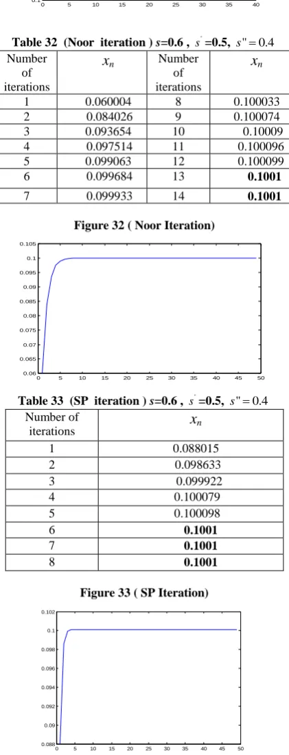
Table 32 (Noor iteration ) s=0.6 , '
s =0.5, s"0.4 Number
of iterations
x
n Numberof iterations
x
n1 0.060004 8 0.100033
2 0.084026 9 0.100074
3 0.093654 10 0.10009
4 0.097514 11 0.100096
5 0.099063 12 0.100099
6 0.099684 13 0.1001
7 0.099933 14 0.1001
Figure 32 ( Noor Iteration)
0 5 10 15 20 25 30 35 40 45 50
0.06 0.065 0.07 0.075 0.08 0.085 0.09 0.095 0.1 0.105
Table 33 (SP iteration ) s=0.6 , '
s =0.5, s"0.4 Number of
iterations
x
n1 0.088015
2 0.098633
3 0.099922
4 0.100079
5 0.100098
6 0.1001
7 0.1001
8 0.1001
Figure 33 ( SP Iteration)
0 5 10 15 20 25 30 35 40 45 50
0.088 0.09 0.092 0.094 0.096 0.098 0.1 0.102
0 5 10 15 20 25 30 35 40
[image:8.595.58.278.63.688.2] [image:8.595.59.536.68.672.2] [image:8.595.323.534.200.750.2]Number of
iterations
x
n1 0.100025
2 0.1001
3 0.1001
4 0.1001
5 0.1001
Figure 34 (Agarwal et al. iteration)
0 5 10 15 20 25 30 35 40
0.1 0.1 0.1 0.1001 0.1001 0.1001 0.1001 0.1001 0.1001 0.1001
Table 35 (Noor Iteration) s = 0.6 , '
s = 0.8, s"0.7 Number
of iterations
x
n Numberof iterations
x
n1 0.060025 8 0.100034
2 0.084053 9 0.100074
3 0.093674 10 0.10009
4 0.097527 11 0.100096
5 0.09907 12 0.100099
6 0.099688 13 0.1001
7 0.099935 14 0.1001
Figure 35 (Noor Iteration)
0 5 10 15 20 25 30 35 40 45 50
0.06 0.065 0.07 0.075 0.08 0.085 0.09 0.095 0.1 0.105
Table 36 (SP Iteration) s=0.6, '
s =0.8, "s 0.7 Number of iterations
x
n1 0.097655
2 0.10004
3 0.100099
4 0.1001
5 0.1001
Figure 36 (SP iteration)
0 5 10 15 20 25 30 35 40 45 50
0.0975 0.098 0.0985 0.099 0.0995 0.1 0.1005 0.101
4. OBSERVATIONS
From comparative analysis (in the form of tables and graphs) we observe that in case of quadratic polynomial for
(i) s=0.6, '
0.1, " 0.1
s s
(ii) s=0.6, '
0.3, " 0.1
s s
(iii) s=0.6, '
0.5, " 0.4
s s
the decreasing order of convergence rate of iterative schemes is as follows:
Agarwal et al. , SP and Noor iterative scheme. But for s = 0.6, '
0.8, " 0.7
s s the decreasing order of convergence of iterative schemes is as follows:
SP, Agarwal et al. and Noor iterative scheme.
Also in case of cubic and biquadratic polynomial the decreasing order of convergence of iterative schemes is Agarwal et al., SP and Noor iterative scheme for all above mentioned cases.
5. CONCLUSION
Keeping in mind comparative analysis drawn by Rana, Dimri and Tomar[1], Tables 1-36 and observations in section 4 we conclude that
(i) In case of quadratic polynomial for 0 < s < 1,
' 1
0 , " 2 s s
, the decreasing order of convergence of
iterative schemes is as follows :
Picard, Agarwal et al., SP, Noor, Ishikawa and Mann iterative scheme.
For 0 < s < 1, ' 1
0 , " 2 s s
, Picard and Agarwal et al.
iterative schemes shows equivalence while the decreasing order of convergence of iterative schemes is as follows : SP, Agarwal et al., Mann, Noor and Ishikawa iterative scheme.
(ii) In case of cubic polynomial for 0< s <1, ' 1
0 , " 2 s s
,
the decreasing order of convergence rate of iterative schemes is as follows :
Picard, Agarwal et al., SP, Noor, Ishikawa and Mann iterative scheme.
For 0 < s <1, 0 < ' 1
" 2
s s Picard and Agarwal et al. schemes shows equivalence while decreasing order of convergence of iterative schemes is as follows :
Agarwal et al., SP, Ishikawa, Noor and Mann iterative scheme.
For 0 < s < 1, ' 1
0 , " 2 s s
, the decreasing order of
convergence rate of iterative schemes is as follows :
Agarwal et al., SP, Mann, Ishikawa and Noor iterative scheme while Picard and Agarwal et al. schemes shows equivalence.
(iii) In case of biquadratic polynomial for 0 < s <1,
' 1
0 , " 2 s s
, Picard and Agarwal et al. schemes shows
equivalence and the decreasing order of convergence rate of iterative schemes is as follows :
Agarwal et al., SP, Noor, Ishikawa and Mann iterative scheme .
For 0 < s < 1, ' 1
" 2
[image:9.595.61.275.69.764.2]Agarwal et al., SP, Ishikawa, Noor and Mann iterative scheme.
For 0 < s <1, ' 1
0 , " 2 s s
, the decreasing order of
convergence rate of iterative schemes is as follows :
Agarwal et al., SP, Mann, Ishikawa and Noor iterative scheme while Picard and Agarwal et al. schemes shows equivalence. Hence, in case of polynomial functions in complex space,
Picard scheme is best for 0 < s <1, ' 1
0 , " 2 s s
while for 0< s
<1, ' 1
0 , " 2 s s
, Agarwal et al. iterative scheme can have
better convergence rate than the other iterative schemes. Futhermore, we conclude that with the increase in power of polynomial, convergence rate of all iterative schemes increase rapidly.
ACKNOWLEDGEMENTS
The authors would like to thank the referee for his/her valuable comments and suggestions.
REFERENCES
[1] Rana, R., Dimri, R. C. and Tomar, A. 2011 Remarks on convergence among Picard , Mann and Ishikawa iteration for complex space, volume 21, no 9 , May 2011 .
[2] Rhoades, B. E. 1976 Comments on two fixed point iteration methods, Journal of Mathematical Analysis and Applications, vol. 56, no. 3, pp. 741-750.
[3] Singh, S. L. 1998 A new approach in numerical praxis, Progress Math.(Varanasi) 32(2), 75-89.
[4] Berinde, V. 2004 Picard iteration converges faster than Mann iteration iteration for a class of quasi-contractive operators, Fixed Point Theory and Applications 2, 97-105.
[5] Berinde, V. 2007 Iterative Approximation of Fixed Points, Editura Efemeride.
[6] Hussian, N., Rafiq, A., D, Bosko and L. Rade 2011 On the rate of convergence of various iterative schemes, Fixed Point Theory and Applications 45,6 pages
[7] Phuengrattana, W., Suantai, S. 2011 On the rate of convergence of Mann, Ishikawa, Noor and SP iterations for continuous functions on an arbitrary interval, Journal of Computational and Applied Mathematics, 235, 3006- 3014.
[8] Mann, W. R. 1953 Mean value methods in iteration, Proceedings of the American Mathematical Society, vol.4, pp. 506-510.
[9] Ishikawa, S. 1974 Fixed points by a new iteration method, Proceedings of the American Mathematical Society, vol. 44, no. 1, pp. 147-150.
[10]Agarwal, R.P., O’Regan, D. and Sahu, D.R. 2007 Iterative construction of fixed points of nearly asymptotically nonexpasive mappings, Journal of Nonlinear and Convex Analysis 8(1),61-79.