https://doi.org/10.5194/jsss-7-57-2018
© Author(s) 2018. This work is distributed under the Creative Commons Attribution 4.0 License.
An SQP method for Chebyshev and hole-pattern fitting
with geometrical elements
Daniel Hutzschenreuter1, Frank Härtig1, and Markus Schmidt2 1Abteilung Mechanik und Akustik, Physikalisch-Technische Bundesanstalt (PTB),
Braunschweig, 38116, Germany
2Werth Messtechnik GmbH, Gießen, 35394, Germany
Correspondence:D. Hutzschenreuter ([email protected])
Received: 3 July 2017 – Accepted: 1 December 2017 – Published: 6 February 2018
Abstract. A customized sequential quadratic program (SQP) method for the solution of minimax-type fitting applications in coordinate metrology is presented. This area increasingly requires highly efficient and accurate algorithms, as modern three-dimensional geometry measurement systems provide large and computationally intensive data sets for fitting calculations. In order to meet these aspects, approaches for an optimization and parallelization of the SQP method are provided. The implementation is verified with medium (500 thousand points) and large (up to 13 million points) test data sets. A relative accuracy of the results in the range of 1×10⁻¹⁴is observed. With four-CPU parallelization, the associated calculation time has been less than 5 s.
1 Introduction
Three-dimensional coordinate metrology is an essential el-ement of modern economic production. The application of coordinate measuring machines (CMMs) offers an efficient way to inspect geometrical properties of workpieces. The manufactured workpieces are measured in a first step. Then, through the mathematical fitting of ideal geometrical ele-ments to the measured features, an evaluation of workpiece deviations from the nominal shape in a technical drawing is possible. The information generated on the deviations is used to classify workpieces as, for example, scrap parts and to ad-just the manufacturing parameters in order to reduce the per-centage of non-permissible parts in the production process.
Optical and computer tomography (CT) measurement systems have gained increasing importance for three-dimensional coordinate metrology in recent years. The rapid development of new applications and measurement capabili-ties poses a great challenge for developers of CMM software as well as for metrological institutes to provide traceability for different measurands. Fitting software has to keep up with an increasing amount of measurement data and simultane-ously the accuracy of calculation results needs to meet high requirements. Under these conditions, PTB (Physikalisch-Technische Bundesanstalt) together with the German CCM
manufacturer Werth Messtechnik GmbH have developed a sequential quadratic program (SQP) for the calculation of Chebyshev and hole-pattern fitting applications with differ-ent geometrical elemdiffer-ents. Through very simple modifitions and computational parallelization, this method is ca-pable of highly accurate and efficient calculations with large data sets as necessary for optical and CT measurements of workpieces in manufacturing.
ap-proximation. However, a significant higher accuracy of fit-ting results can be achieved. Furthermore, the QP decent directions provide quadratic or at least super linear conver-gence speed of the method, which is an advantage compared to a linear approach.
The input for the Chebyshev and hole-pattern fitting is a point data set:
P = {P1, . . ., Pm},
wherePi= Pix, Piy, PizT∈R3(i=1, . . .m) are Cartesian coordinates of points on the surface of a real workpiece. The ideal geometrical element for the fit is defined by a number of parameters:
a=(a1, . . ., an−1)T∈Rn−1.
These give either the geometrical element parameters in the case of Chebyshev applications, or transformation parame-ters in the case of hole-pattern fitting. In general, the param-eter values are overestimated as the amount of measurement pointsmis much larger than the numbern−1 of unknown parameters. Hence, the fit considers the orthogonal distances,
fi(a),
between the points Pi∈P and the ideal geometry with
pa-rametersa. The model for the calculation of the geometrical parameters is then the minimax program
mina∈Rn−1maxi=1,...,mfi(a). (1)
The objective is to find parameter values for a that mini-mize the maximum orthogonal distance between all points and the geometrical element. For the development of SQP methods, program (1) is equivalently transformed into an or-dinary non-linear constrained form.
minv∈Rnf(v) (2)
subject togi(v)≤0 (i=1, . . ., m)
hj(v)=0 (j =1, . . ., q)
Here, v:= aT, sT
∈Rn denotes the extended parameter vector. The new parametersis an upper bound for the maxi-mum over allfi(a) in program (1). By introducingf(v):=s
as an objective and the set of inequality constraintsgi(v):=
fi(a)−s, it equivalently replaces the minimization of the
maximum term. The equality constraintshj(v) complete the
model and implement additional conditions related to the definition of the parameter vectora.
Section 2 gives the SQP core algorithm. It subsequently requires the application of a solver for quadratic programs. An optimized quadratic program solver for the fitting ap-plications of interest is given in Sect. 3. For specific non-regular solutions of program (2), a second-order criterion for a solution is presented in Sect. 4. The numerical precision of
calculations by the customized SQP method is then investi-gated in Sect. 5 using the example of flange ring inspections (Hutzschenreuter et al., 2017) that require different types of minimax fits to be calculated. Finally, the effect of the par-tial parallelization of the algorithm and the resulting runtime improvements are investigated in Sect. 6.
2 The SQP method
For the application of an SQP method, the Lagrangian of program (2) is considered. For the Lagrange multipliersλ=
(λ1, . . ., λm)T∈Rmandµ= µ1, . . ., µqT∈Rq, it is
L(v,λ,µ):=f(v)+Xm
i=1λigi(v)+
Xq
j=1µjhj(v).
Under the assumption of a regularity constraint qualification (e.g. the linear inequality constraint qualification; Geiger and Kanzow, 2002), a local minimum of (2) and its Lagrangian have multipliers for which the Karush–Kuhn–Tucker (KKT) condition
∇vL(v,λ,µ)=0 (3)
hj(v)=0 (j=1, . . ., q)
gi(v)≤0,λi≥0,λigi(v)=0 (i=1, . . ., m)
is satisfied. The SQP method is derived from this nec-essary condition by applying a Lagrange–Newton method to ∇vL(v,λ,µ)=v, hj(v)=0(j=1, . . ., q) and gi(v)≤
0 (i=1, . . ., m).
Algorithm 1 (globalized SQP method)
(S0) Set initial values forv0,λ0,µ0,α >0,β∈(0,1),σ ∈
(0,1)andH0=In∈Rn×n,k=0. (S1) If vk,λk,µk
satisfy KKT condition (3), stop.
(S2) Calculate a decent direction1v∈Rnand λk+1,µk+1
from the quadratic program
min1v∇vfvkT1v+ 1
21v
TH
k1v subject to (4)
gi
vk+ ∇vgi
vkT1v≤0 (i=1, . . ., m)
hj
vk+ ∇vhj
vkT1v=0 (j=1, . . ., q).
Ifk1vk =0,stop with solution vk,λk+1,µk+1.
(S3) Calculate a step width tk≥0 (tk=βl, l=0,1,2, . . .)
that satisfies
P1
vk+tk1v, α
≤P1
vk, α−tkσ P10
vk,1v, α. (5)
In Algorithm 1, the matrixHk is a positive semi-definite
approximation of the Lagrange function’s Hessian. It guaran-tees that the quadratic program (4) in step (S2) has a solution. Its update is made with the Broyden–Fletcher–Goldfarb– Shanno method (BFGS, Geiger and Kanzow, 2002).
The initial values for the parameter vector shall be a fea-sible point of the minimization program. Such a point satis-fies the constraints gi v0≤0 (i=1, . . ., m) and hj v0=
0 (j =1, . . ., q). The initial Lagrange multiplier values are selected as zero values. In each iteration of the algorithm, the update of the Lagrange multipliers is calculated by solv-ing the QP in step (S2). Thereby,λk+1andµk+1are the
La-grange multipliers associated with program (4). Details on their definition are presented in the following section.
In step (S3) formula (5), the Armijo-type step width is cal-culated from the exactl1-barrier-penalty function.
P1(v, α):=f(v)+α
nXm
i=1max{0, gi(v)} +Xq
j=1
hj(v)
o
The termP10(vk,1v, α) is its directional derivative invk to-wards1v. Step (S3) is a commonly used globalization tech-nique for enabling the super-linear convergence up to the quadratic convergence of the SQP method towards a solution of the KKT system (3). Parameter αcontrols the influence of invalid constraints on the step width;βis the basis for the Armijo steps andσ adds some additional damping.
3 Customized active-set QP method
Solving the QPs (4) in step (S2) of the SQP method is the most time-consuming part when considering fitting large data sets. The applied algorithm is an active-set method, which overcomes the efficiency problem by introducing sim-ple modifications. A minimum of program (4) defines the ac-tive set of inequality constraints that are equal to zero.
A:=
i∈ {1, . . ., m} |gi(v)+ ∇vgi(v)T1v=0
Through gA∈R|A|, a vector is introduced whose compo-nents are gi vk with i∈A. The matrix GA∈R|A|×n has the rows∇vgiT(vk) for alli∈A. Finally,hdenotes a vector whose components are all hj(vk) andHis the matrix with
the columns∇vhTj(vk) (j =0, . . ., q). The KKT condition for a local solution of program (4) introduces the Lagrange mul-tipliersλA∈R|A| for all the active constraints and µ∈Rq for the equality constraints.
With these preliminary definitions for linearly independent
∇vgiT vk(i∈A) and ∇vhTj(vk) (j =0, . . ., q), the KKT
condition for QP (4) is
Hk GTA HT
GA 0 0
H 0 0
1v λA µ =
−∇vf vk
−gA −h (6) gi
vk+ ∇vgi
vkT1v <0 (i6∈A) λi≥0 (i∈A), λi =0 (i6∈A)
The following algorithm uses approximations Al of A and
the KKT condition (6) to calculate a solution of program (4). It uses iteratively calculated approximations of1v with the indexl=0,1,2, . . .that are
1vl:=
1alT, 1sl
T
=1a1l, . . ., 1aln−1, 1sl
T
.
Algorithm 2 (customized active-set method for QP)
(S0) Forl=0,calculate initial values1v0, A0,λA0 andµ by solving
In HT
H 0 1v∗ µ0 = 0 −h (7)
1a0= 1v1∗, . . ., 1v∗n−1T
1s0= max
i=1,...,m
gi
vk+ ∇vgi
vkT1v∗
1v0=1a0, 1s0
T
A0=
i|gi
vk+ ∇vgi
vkT1v0=0
λi1 (i∈A0),
λi=0 (i6∈A0)
and
µ=µ0.
(S1) If 1vl,λ Al,µ
satisfies KKT condition (6), stop. (S2) Calculate an update directiond by solving the linear system
Hk GTAl H T
GAl 0 0
H 0 0
d λAl
µ (8) =
−∇vf vk
−Hk1vl 0
0
(S3) Ifkdk =0
(S3.1) Ifλi≥0 for all i∈Al, stop with the solution 1vl,λ
Al,µ
from (8).
(S3.2) Otherwise createAl+1fromAl by removing the
(S4) Ifkdk 6=0
(S4.1) If gi vk+ ∇vgi vk T
(1vl+d)≤
0 (i=1, . . ., m),set1vl+1=1vl+dandA
l+1=Al.
(S4.2) Otherwise calculate
Ki:=
gi(vk)− ∇vgi(vk)T1vl ∇v
gi(vk)Td
(i=1, . . ., m),
t=mini6∈Al
n
Ki
∇vgi(v
k)T1vl>0o
and set1vl+1=1vl+td, Al+1=Al∪ {j}.
(S5) Setl=l+1and go to step (S1).
The initialization step (S0) is a specific customization of the method that speeds up the calculations significantly. Both vector 1a0 and1s0 are derived from the solution 1v∗ of the linear equation system (7). These values satisfy the con-straints of QP (4). It is only applicable for the minimax fitting models (1) and respectively for its transformation (2).
For large data sets, the degeneration of the linear equation system (8) may occur. Then some of the active constraint columns become linearly dependent and a unique solution of the update direction d is not available. Through a heuristic approach, the system matrix in Eq. (8) is extended by the regularization term −ρ3 gA
l
, which is a diagonal matrix with the components ofgA
l weighted with 0< ρ1. The equation system that is solved instead of Eq. (8) is as follows.
Hk GTAl H
T GAl −ρ3 gAl
0
H 0 0
d λAl
µ
(9)
=
−∇vf(vk)−Hk1vl 0
0
If in subsequent iterations of Algorithm 2 (8) is degener-ated, the calculation is stopped and a non-optimal solution for1v=1vlis returned to the SQP method.
Furthermore, a maximum for the iteration indexl should be set to guarantee the finite termination of the method. If the maximum index is reached, a non-optimal solution is also returned to the SQP.
Note that a solution 1vl,λ Al,µ
from Algorithm 2 pro-vides the Lagrange multipliers for the next SQP iteration
µk+1=µ,λk+1
i =0 (i6∈Al), andλ k+1
i is the corresponding
value fromλAl for alli∈Al.
4 Second-order sufficiency condition
The aim of applying a second-order sufficiency condition is to verify that a solution of the SQP algorithms is a valid min-imum of the fitting program (2). For this purpose, the follow-ing theorem form (1) is utilized.
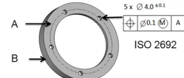
Figure 1.Nominal flange model and measured (extracted) features.
Theorem (second-order sufficiency condition)
Let(v,λ,µ)be a solution of (2) that satisfies KKT condition (3). If
zT∇vvL(v,λ,µ)z>0 (10)
holds for allz∈Rn,z6=0with
∇vgi(v)Tz=0 for alli∈Awithλi >0 ∇vgi(v)Tz≤0 for alli∈Awithλi=0
and
∇vhj(v)Tz=0 for allj =1, . . ., q
then the solution is a strict minimum of the fitting application.
Computationally, condition (10) can be treated by a quadratic program and by minimizing zT∇vvL(v,λ,µ)z.
The application of Algorithm 2 is valid. In the implementa-tion, the Hessian is approximated by central difference quo-tients. The active setA and the Lagrange multipliers λ,µ
used in the theorem above are those from the last QP itera-tion in Algorithm 1.
Condition (10) implies that the Hessian matrix
∇vvL(v,λ,µ) of the Lagrangian is positive definite on the orthogonal complement of the affine subspace in Rn, which is spanned by the gradients of active constraints with positive Lagrange multiplier values and the gradients of the equality constraints. Its application is necessary for special data sets where active constraints haveλi=0 or where the
number of linearly independent active constraint gradients and equality constraint gradients is less thann.
5 Test calculations
Figure 2.Extracted flange.
into the holes. The alignment of the virtual counterpart to the holes is constrained by the datum elements A (Chebyshev plane) and B (minimum-circumscribed cylinder). A CMM measures points on the inner surface of all clearance holes and on the surfaces A and B. The data are denoted as the extracted workpiece and outlined in Fig. 2.
The extracted geometry of plane A is outlined by large round dots. These give the measurement pointsP1P, . . ., PmP
p. Points P1C, . . ., PmC
C are the extracted cylinder surface B which is marked by rectangular dots in Fig. 2. Finally, the small round dots outline the geometry measured in the holes. These have the point setsP1k, . . ., Pmkk, wherek is a unique index for each hole.
In the first calculation step, datum plane A is fitted to the extracted flange. The fitting model is
min maxi=1,...,mP
fi CP,
− →
n (11)
subject to
− →
n
=1,(G−CP)T − →
v =0∀−→v ⊥−→n.
The amount of points for the plane is mP. The
geometri-cal parameters are the pointCP on the plane and its normal
vector−→n;fi(CP,−→n) is the orthogonal distance between the
pointPiP and the plane associated withCP,−→n. Furthermore,
the geometrical parameters have two constraints. The length of the normal vector must be one. The point on the plane is defined as the orthogonal projection of the extracted plane centroidG=1/mP Pmi=P1P
P i
on the associated plane. In the SQP method, it is implemented by constructing two non-parallel vectors −→v1,
− →
v2 that are orthogonal to − →
n and by considering the equality constraints (G−CP)T
− →
v1=0 and
(G−CP)T − →
v2=0.
In the second calculation step, the minimum-circumscribed cylinder is fitted to the extracted outer surface B. The axis direction of the associated cylinder is constrained to be parallel to the plane normal vector that was calculated before. Then the fitting model is
min maxi=1,...,mCfi(CC) (12)
subject to (CP−CC)T − →
n =0.
The geometrical parametersCCfor the fit are the coordinates
of a point on the cylinder axis. Here, fi(CC) gives the
or-Figure 3.Associated Chebyshev plane (element with dashed edges)
and minimum-circumscribed cylinder (element with dash-dotted edges) for the flange.
Figure 4.Hole-pattern fit of the flange. In the actual alignment, the
gauge overlaps with the extracted workpiece which is outlined by the black dots intersecting with the circular gauge elements.
thogonal distance between the cylinder axis and the pointPiC on the extracted surface B. Furthermore, the position of the cylinder axis is constrained to be an element of the associated plane A.
Figure 3 shows an outline of the associated plane and cylinder. The point CC and normal vector −→n are
used to specify a Cartesian workpiece coordinate system (xW, yW, zW). The direction of thezaxis is defined by−→n.
All the Cartesian axes intersect inCC.
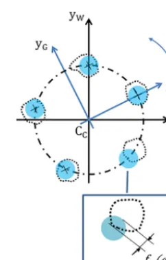
In the last calculation step, the hole-pattern fit of the clear-ance holes is calculated. Figure 4 shows the fitting of the gauge and the extracted geometry in parallel projection onto thex–yplane of the workpiece coordinate system.
The virtual counterpart for the fit represents five cylin-ders that are the solid circular elements in Fig. 4. Their axes are parallel to thezaxis of the Cartesian coordinate system (xG, yG, zG), which is denoted as a gauge coordinate system.
coor-dinate system in the centre pointCCand withzGparallel to
zW. At fitting, the whole gauge coordinate system and the
counterpart elements are rotated around thezaxis by the an-gleϕ. If there is one position where all cylinder elements fit into the extracted holes and no point overlaps with the inside of the cylinders, the flange ring is within its tolerance for the maximum permissible shape deviations. The minimax pro-gram for the calculation of such an angle is
min max k=1,...5 i=1,...,mk
fki(ϕ). (13)
Herekis an index that uniquely identifies each clearance hole and its associated element of the counterpart. Number mk
gives the amount of measurement points for each hole. The orthogonal distancefki(ϕ) between the outer surface of the
cylinder with the indexkand the pointPik is positive if the point is inside the cylinder (overlapping). Otherwise the dis-tance has a negative value. All cylinder elements and hence the virtual counterpart fit into the clearance holes at the same time if
s:=maxk=1,...5 i=1,...,mk
fki(ϕ)≤0 (14)
at a solution of program (13).
In order to investigate the precision of the customized SQP method for the calculations (11), (12) and (13) of the flange ring inspection, test data sets DS1, . . . , DS6 were created by an inverse data generator. It relies on the state-of-the-art methods in Anthony et al. (1993), Forbes and Minh (2012) and Hutzschenreuter et al. (2015). Each data set refers to a nominal flange with ten clearance holes of ra-dius 5 mm, an outer ring rara-dius of 120 mm and a height of 20 mm. A reference solution of the flange fit is input for the data generator. It is given by the gauge coordinate system CR,xRGyRGzRGand the maximum distancesRfor the solution
of program (12). The generator then computes positions of measurement points that give a test data set for which the reference parameters represent the unambiguous global min-imum of fitting. The points differ from the nominal shape of the flange by a random uniform form deviation. All points are equally distributed along rectangular surficial grids on the nominal flange surface. It simulates the dense probing from optical or likewise CT-sensor-based measurements. The gauge coordinate systemCR, xGRyRGzRGandsC from the
cal-culation with the SQP method is compared to the reference coordinate system according to Fig. 5.
The deviations between both coordinate systems are cal-culated by
ds:=
s
R−sC
dC:= kCR−CCk
α:=
x
R G×x
C G
β:=
y
R G×yGC
Figure 5.Principle of the comparison between reference and
cal-culated gauge coordinate systems.
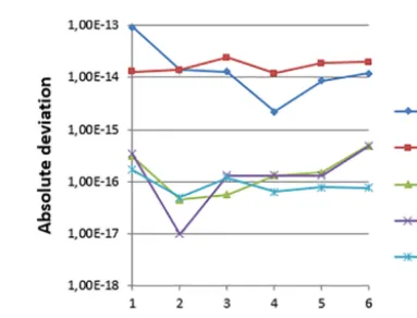
Figure 6.Deviation of the calculated flange fit to the reference
so-lution.
γ:=
z
R G×z
C G.
Calculations for the six data sets were made with an absolute convergence tolerance for the SQP steps of 1×10⁻¹⁴. The
algorithm is implemented in C++(full compiler optimiza-tion, Microsoft Visual Studio, 2013), double precision float-ing point number format (IEEE 754, 2008). Figure 6 presents the deviations of the computed fit to the reference solution.
For all data sets, the SQP method converged to a solu-tion of the flange ring fitting. The maximum distance devi-ationdsand the gauge coordinate system position deviation dCare between 1×10⁻¹³ and 1×10⁻¹⁵mm, which corre-sponds to the convergence tolerance. Similarly, the deviation of all coordinate system axes is of the size 1×10⁻¹⁶rad. This deviation is in the size of the relative machine preci-sion of real number representation in floating point arith-metic (IEEE 754, 2008). In conclusion, the SQP method was able to calculate highly numerically precise solutions for the flange ring fitting examples.
for the maximum of SQP iterations and QP iterations are set to ensure the finite termination of the algorithm. For the flange these are 100 SQP iterations. The number of QP it-erations is, in comparison, set to a maximum of 10 for the Chebyshev plane and hole-pattern fit as well as 20 for the MC cylinder. If the QP method does not converge to a so-lution within the given number of iterations, then the SQP method continues with a non-optimal decent direction which has no significant influence on the overall convergence of the algorithm. The step-width control parameters are set toα=1 for all fitting applications. It allows large decent steps which violate boundary constraints. All violations are corrected by the initial value selection of each subsequent QP method call. This approach bypasses slow convergence properties like the Maratos effect (Geiger and Kanzow, 2002). In addition, the step scaling parameter was set toβ≥0.7 and the maximum number of Armijo steps is 2, which forces large steps in each SQP iteration.
Further verification of the customized SQP method was made by using the public test for Chebyshev geometrical el-ements of PTB (Hutzschenreuter et al., 2015). Calculations were made for 50 different geometrical element data sets. The elements covered by the test are a two-dimensional cir-cle, two-dimensional straight line, plane sphere and cylinder. In comparison to the previously used flange ring data sets the Chebyshev test data sets also simulate the effect of system-atic form deviations such as harmonic deviations and con-vexity as well as full and partitial features. In these cases it is more likely that an insufficient implementation of an fit-ting algorithm will end up in an local minimum which is not the required fitting solution. For all elements in the test, the initial values for the Chebyshev fitting were calculated by Gaussian fitting. Conveniently, the implementation of the Gaussian fitting is possible with the SQP method. Only the convergence speed towards a solution is very slow for this non-minimax-type fitting. With these preliminaries the pub-lic Chebyshev element test was passed for all 50 test data sets with an maximum permissible error of 0.1 µm for position and size parameters, 0.01 µm for form deviation and 0.1 µrad for the orientation of the geometrical element parameters.
Finally, the following additional test calculations point out the effect of outliers in the given measurement data sets and the influence of different selections of initial values for the SQP method.
Outliers denote perturbations in the measurement data of the extracted geometry that can occur when dirt particles such as dust stick to the workpiece surface at the measure-ment. A reliable evaluation of the geometrical measurands requires removal of these outlier points form the data before applying Chebyshev and hole-pattern fitting as they have a considerable influence on the solution of fitting program (1). The situation is outlined for the flange data set DS1. Mea-surement pointP1P of the datum plane is shifted step-wise by settingP1P =P1P+a·−→n witha=0,0.1,0.2, . . .,1. Thereby, the normalnis the direction given by the reference plane fit
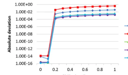
Figure 7.Deviation between the calculated flange fit and the
ref-erence solution for a simulated outlier point in the extracted plane data set.
of the test data set. The resulting deviation between reference flange fit and the fit with the SQP method is shown in Fig. 7. The deviation of the fitting solution is strongly correlated with the shift ofP1P. Fora≥0.3 mm the deviation of the fitting parametersof the hole-pattern fit becomes larger than 0.01 mm. In this case the solution of the SQP method changes from the virtual gauge fitting into all holes to an overlapping. The workpiece would be identified as out of its tolerance only because of the presence of one outlier.
The choice of an initial solutionv0affects the calculation time of the SQP method and whether the algorithm converges to the global fitting minimum or to some inadequate local solution. For the Chebyshev plane fit in program (11) it is sufficient to select the gravity centre point of the given mea-surement data as initial position. An initial normal can be drawn from a list of candidate direction vectors as the nor-mal direction that provides the snor-mallest form deviation with the initial centre point. Similarly the initial approximation for the MC cylinder in program (12) can be the fitting result of the Chebyshev plane. For the hole-pattern fit a more sophis-ticated method is required to determine an initial rotationϕ0 of the virtual gauge. An example is the Gaussian centre-point fit presented in Hutzschenreuter et al. (2017). It provides fast convergence for the flange fit examples. The effect of choos-ing different initial values for the hole-pattern fit is shown in Fig. 8.
Figure 8.Effect of a variation of the initial value for the flange hole-pattern fit on the calculated SQP solution and its performance with DS1.
cases. Ford= −1,−0.8,−0.4 andd=1 the SQP method converges to different local solutions that give a wrong fit-ting result. These calculations have up to 50 SQP iterations and more than 350 QP iterations. Moreover, all calculations show that the QP method has the greatest share of the total calculation time. In the best case withd=0, the SQP method requires only four iterations to converge to the global mini-mum with relative precision, as shown in Fig. 6. The amount of QP iterations is 10. In the worst case – with a correct so-lution – 28 SQP iterations and 214 QP iterations have been counted atd=0.8. Especially for data sets with uneven size ratios such as long cylinder elements or partitial features, the area for fast convergence of the SQP method becomes more narrow than in the test examples DS1–DS6.
6 Parallelization
The efficiency of the calculation is improved by the partial parallelization of the Algorithms 1 and 2. What is suitable for parallelization is the computation of orthogonal distance values and their gradients as well as expensive vector opera-tions that frequently have to be made within the QP active-set method. Due to the iterative structure of the SQP method and the QP active-set method, the basic part of the algorithms re-mains serial. Hence, it is expected that the speedup will not be proportional to the amount of available threads for parallel calculation (e.g. available CPU cores).
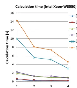
The times in Fig. 9 were measured for calculations of the flange ring fit to data sets DS1, . . . , DS6 of the previous section at a workstation with an Intel(R) W3550 CPU and absolute convergence tolerance 1×10⁻¹⁴. For all data sets, the speedup for four threads is approximately between fac-tor 3 and facfac-tor 4 compared to the serial computation with 1 thread. The fit for the small and medium-sized data sets DS1, . . . , DS4 (up to 6 million points) is less than 1 s for four thread calculations. The speedup decreases with an increas-ing amount of threads.
Figure 9.Calculation times for flange ring fitting with different
amounts of parallel threads.
7 Conclusions
Minimax-type fitting applications in coordinate metrology such as Chebyshev, minimum-circumscribed, maximum-inscribed and hole-pattern fitting can be transformed into a convenient general non-linear constrained form. For this for-mulation of the applications, a very efficient solver was de-veloped from a basic SQP method by means of simple mod-ifications. For flange ring fitting test data sets, the software was able to compute highly numerically precise solutions with a relative deviation of 1×10⁻¹⁴of the numerical values
from the reference solutions. In addition, a verification with TraCIM Chebyshev element test data sets was made.
standard even for office computers. Subsequently, the perfor-mance capacity of modern multicore workstation CPUs (8, 16 and more cores) can almost fully be exploited for further reduction of the calculation time.
In further metrological applications, the SQP method is suitable for the simulation of numerical uncertainties of ge-ometrical element and fitting calculation results by Monte Carlo methods (JCGM, 2008). Moreover, due to its accu-racy, it can be used for the validation of data sets from in-dustrial test services – for example the TraCIM validation service (PTB, 2015).
Finally, one aim is to provide the software to users of CMM as part of the WinWerth evaluation software of-fered by the multi-sensor CCM manufacturer Werth (Werth Messtechnik GmbH, 2017). An implementation is provided for different three-dimensional hole-pattern fitting applica-tions such as the calculation for the flange ring. Further details are given in the PTB hole-pattern fitting guideline (Hutzschenreuter et al., 2017).
Data availability. The authors’ original test data are available at
Appendix A: Test data set properties
The rotation angles Rx,Ry and Rz in Table A2 refer to a
rotation of the gauge (virtual counterpart of hole-pattern fit) around the coordinate system axes. Each rotation is clock-wise. First the gauge is rotated around thezaxis. A rotation around theyaxis and finally around thexaxis follow.
Table A1.Amount of measurement points per test data set.
Calculation DS1 DS2 DS3 DS4 DS5 DS6
MZ plane 70 104 140 642 281 460 563 620 1 128 094 2 257 450 MC cylinder 69 960 139 922 279 994 559 860 1 119 987 2 239 784 Hole pattern 259 840 519 470 1 038 280 2 079 990 4 158 260 8 316 880 Total 399 904 800 034 1 599 734 3 203 470 6 4063 41 12 814 114
Table A2.Reference solutions for hole-pattern fit of test data sets.
Parameter DS1 DS2 DS3 DS4 DS5 DS6
Cx[mm] +10.00
Cy[mm] −20.00
Cr[mm] +42.00
Rx[rad] 0.500 0.510 0.490 0.490 0.490 0.520
Ry[rad] −0.130 −0.120 −0.120 −0.120 −0.130 −0.140
Rz[rad] 0.034 0.044 0.044 0.044 0.024 0.024
s[mm] −0.012
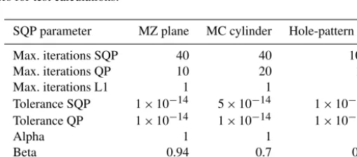
Appendix B: SQP solver parameters
Table B1.SQP method parameters for test calculations.
SQP parameter MZ plane MC cylinder Hole-pattern fit
Max. iterations SQP 40 40 100
Max. iterations QP 10 20 10
Max. iterations L1 1 1 2
Tolerance SQP 1×10⁻¹⁴ 5×10⁻¹⁴ 1×10⁻¹⁴ Tolerance QP 1×10⁻¹⁴ 1×10⁻¹⁴ 1×10⁻¹⁴
Alpha 1 1 1
Beta 0.94 0.7 0.7
Gamma 0.9 0.9 0.9
Competing interests. This paper and its content, numbers and figures were authorized for publication by M. Schmidt, who is co-author and leader of the software development department of Werth Messtechnik GmbH.
Acknowledgements. This research is funded by the German
Federal Ministry of Economic Affairs and Energy and Werth Messtechnik GmbH within the scope of the MNPQ-Transfer project “3D-Lochbildeinpassung für Koordinatenmesssysteme mit taktilen und optischen Sensoren sowie CT-Systemen”.
Thanks go to Matthias Franke from PTB for the support provided with numerical calculations and Harald Löwe from the Technical University of Braunschweig for his many helpful remarks which improved the presentation of the algorithms. Finally, the authors like to thank the anonymous reviewers for their many suggestions that helped to improve the understanding of the SQP method and its application.
Edited by: Rainer Tutsch
Reviewed by: two anonymous referees
References
Anthony, G. T., Anthony, H. M., Bittner, B., Butler, B. P., Cox, M. G., Drieschner, R., Elligsen, R., Forbes, A. B., Groß, H., Hannaby, S. A., Harris, P. M., and Kok, J.: Chebychev best-fit ge-ometric elements, Centrum voor Wiskunde en Informatica, Re-port NM-R9317, 1993.
DIN EN ISO 2692: Geometrical product specifications (GPS) – Geometrical tolerancing – Maximum material require-ment (MMR), least material requirerequire-ment (LMR) and reci-procity requirement (RPR) (ISO 2692:2006), German version EN ISO 2692:2007-04, 2007.
Forbes, A. B. and Minh, H. D.: Generation of numerical artefacts for geometric form and tolerance assessment, Int. J. Metrol. Qual. Eng., 3, 145–150, https://doi.org/10.1051/ijmqe/2012022, 2012. Geiger, C. and Kanzow, C.: Theorie und Numerik restringierter Optimierungsaufgaben, Springer, https://doi.org/10.1007/978-3-642-56004-0, 2002.
Hutzschenreuter, D.: Benchmarking data sets for flange hole pattern fitting, Physikalisch-Technische Bundesanstalt (PTB), https://doi.org/10.7795/710.20170606, 2017.
Hutzschenreuter, D., Härtig, F., Wendt, K., Lunze, U., and Löwe, H.: Online validation of Chebyshev geometrical element algorithms using the TraCIM-system, Journal of Mechanical Engineering and Automation, 5, 94–111, https://doi.org/10.5923/j.jmea.20150503.02, 2015.
Hutzschenreuter, D., Härtig, F., and Schmidt, M.: LoBEK 3D – User Guide to 3 D pattern fitting with coordinate measuring machines, 2017 – Version 1, https://doi.org/10.5923.j.jmea.20150503.02, 2017.
IEEE 754-2008: Standard for Floating-Point Arithmetic, IEEE Standards Association, https://doi.org/10.1109/IEEESTD.2008.4610935, 2008. JCGM: 101:2008, Evaluation of measurement data –
Supple-ment 1 to the “Guide to the expression of uncertainty in measurement” – Propagation of distributions using a Monte Carlo method, available at: http://www.bipm.org/utils/ common/documents/jcgm/JCGM_101_2008_E.pdf, (last access: January 2018), 2008.
Mircrosoft Visual Studio Express 2013: available at: https://www. microsoft.com/en-us/download/details.aspx?id=40769, (last ac-cess: January 2018), 2013.
PTB (Physikalisch-Technische Bundesanstalt): The TraCIM service web pages, available at: http://www.tracim.ptb.de (last access: June 2017), 2015.