RESEARCH
Fast approximate STEM image simulations
from a machine learning model
Aidan H. Combs, Jason J. Maldonis, Jie Feng, Zhongnan Xu, Paul M. Voyles and Dane Morgan
*Abstract
Accurate quantum mechanical scanning transmission electron microscopy image simulation methods such as the multislice method require computation times that are too large to use in applications in high-resolution materials imaging that require very large numbers of simulated images. However, higher-speed simulation methods based on linear imaging models, such as the convolution method, are often not accurate enough for use in these applications. We present a method that generates an image from the convolution of an object function and the probe intensity, and then uses a multivariate polynomial fit to a dataset of corresponding multislice and convolution images to cor-rect it. We develop and validate this method using simulated images of Pt and Pt–Mo nanoparticles and find that for these systems, once the polynomial is fit, the method runs about six orders of magnitude faster than parallelized CPU implementations of the multislice method while achieving a 1 −R2 error of 0.010–0.015 and root-mean-square error/ standard deviation of dataset being predicted of about 0.1 when compared to full multislice simulations.
Keywords: Scanning transmission electron microscopy, Convolution, Frozen phonon multislice simulation, High-throughput, Linear regression
© The Author(s) 2019. This article is distributed under the terms of the Creative Commons Attribution 4.0 International License (http://creat iveco mmons .org/licen ses/by/4.0/), which permits unrestricted use, distribution, and reproduction in any medium, provided you give appropriate credit to the original author(s) and the source, provide a link to the Creative Commons license, and indicate if changes were made.
Background
As the uses of scanning transmission electron micros-copy (STEM) in applications of high-resolution materi-als imaging continue to expand, methods for simulating STEM images become increasingly important. Simulated images are often used to verify or provide quantitative interpretations for experimental STEM results in areas such as high-precision two-dimensional measurements [1], electron ptychography [2, 3], atomic electron tomog-raphy [4–8], and three-dimensional imaging of point defects [9–13].
STEM images can be simulated in several ways. The simplest is the convolution method, an incoherent lin-ear image model that convolves the probe point-spread function with simple atomic potentials for the specimen [14]. This method assumes that there is no dynamic scat-tering and no interference between scattered and unscat-tered electrons [15]. Although the convolution method allows images to be computed very quickly, it is only
accurate for very thin samples, and so has seen limited use. The primary simulation methods for most specimens are the Bloch wave method and the multislice method, both of which are much more computationally expensive than the convolution method. The Bloch wave method requires a very large amount of storage when applied to complex structures, particularly those containing defects [14, 16, 17]. The multislice method [14, 18], often imple-mented using fast Fourier transforms [19] is, therefore, more commonly used. The multislice method can require significant computation times, on the order of weeks of central processing unit (CPU) time [O(106 s/image),
where we use O(X) to represent “on the order” of X] to simulate a typical STEM image [20]. With significant par-allelization, this is not a major limitation when calculat-ing just a few images. However, some recent approaches to structure determination require thousands or even millions of images to be simulated. One such approach is the exploration of configuration space required for inverse structure determination from images [21]. For example, Yu et al. used a genetic algorithm to find a structure that best fits an experimental STEM image while minimizing the particle energy [22]. Large numbers
Open Access
*Correspondence: [email protected]
of multislice simulations may also be needed to verify results of calculations performed on large STEM datasets as, for example, in electron tomography [8, 11]. Large simulated STEM datasets are also increasingly used to train machine learning models for more robust and com-putationally efficient STEM simulations: for example, Xu et al. used several thousand Bloch wave simulations to train a series of convolutional neural networks for high-throughput analysis of four-dimensional STEM data [23]. Many efforts have been made to reduce the calcula-tion time of the multislice method. Codes are available that are parallelized to run on multiple CPUs [24, 25], graphics processing units (GPUs) [26–29], or both [20, 30]. Through efficient parallelization and use of GPUs, the necessary computation time for a multislice simula-tion can typically be reduced by 1–2 orders of magni-tude compared to a single CPU calculation [to O(104 s/
image)]. In work by Pryor et al. four GPUs are required to achieve a speedup of about two orders of magnitude [20]. Ophus et al. achieved decreases in simulation computa-tion times by combining elements of the Bloch wave and multislice methods in an approach known as PRISM [31]. In this approach, a Fourier interpolation factor can be adjusted to trade accuracy for computation speed. When GPU parallelized and with the interpolation factor set to prioritize speed, PRISM is approximately 3–4 orders of magnitude faster than a single CPU multislice implemen-tation [O(103 s/image)] [20].
Yu et al. developed a Z-contrast STEM simulation method for gold nanoparticles that applied a pixel-by-pixel correction to images generated using the convolu-tion method [22]. A high-order polynomial (the exact order is not given in the paper) was fitted to a dataset of STEM pixel intensities from a set of corresponding mul-tislice and convolution images of unit cells of varying thickness. The polynomial effectively corrected the con-volution image to better approximate the more accurate multislice image. However, this one-to-one pixel intensity correction has limited accuracy and the potential to ben-efit from additional information that may be available in the convolution image.
In this work, we generalize and extend the approach of Yu et al. by developing and assessing the accuracy and computation time of several one-to-one and many-to-one pixel intensity corrections. The model in this work is based on a multivariate polynomial fit, which is simple to understand and extremely rapid to fit and apply. This is just one of many possible approaches that could be used, including Fourier or spline regression, kernel ridge regression, Gaussian process regression, decision tree regression, standard neural network models, and deep learning convolution network models. These other tech-niques may yield additional accuracy but were beyond
the scope of this initial investigation and represent prom-ising pathways for future work.
The models used as corrections are trained on data-sets of matched multislice and convolution images of Pt and Pt–Mo nanoparticles with varying amorphous/ crystalline character. For the systems we tested, the best models result in simulated STEM images with an aver-age cross validation root-mean-square intensity error of 0.1 (reported as a fraction of the standard deviation of the total data set being predicted) and cross valida-tion 1 −R2 (where R2 is the coefficient of correlation)
error of approximately 0.01–0.015 when compared to full multislice simulations, comparable to other high-speed multislice approximation methods such as PRISM. A convolution image can be generated and a trained model applied to it in just O(10−2) s of CPU time on a
common desktop processor without the use of any paral-lelization or GPUs. Therefore, this method can simulate STEM images approximately five orders of magnitude faster than PRISM (when PRISM is run to yield a com-parable accuracy to our model) and six orders of mag-nitude faster than GPU-parallelized multislice with a modest loss of accuracy. However, the regression model is system dependent, and must be fitted for each system of interest using a training dataset consisting of convolu-tion images and corresponding multislice images of sam-ples representative of the system. Thus, it is best suited for applications which require large numbers of moder-ately accurate Z-contrast STEM simulations of similar systems.
Methods
All the data sets and codes used in this study, including multislice simulated images and machine learning-esti-mated images, are available on Figshare at https ://doi. org/10.6084/m9.figsh are.74289 20.
Dataset
To develop and validate the method, we generated cor-responding convolution and multislice simulated images for sets of Pt nanoparticles, Pt–Mo nanoparticles with ~ 5% Mo, and Pt–Mo nanoparticles with ~ 50% Mo. Each set contained nanoparticles of similar size but vary-ing structure, rangvary-ing from purely amorphous to purely crystalline. The Pt set contained 20 nanoparticles, each containing 561 Pt atoms. The Pt–Mo 5% set contained 20 nanoparticles, each containing 557 Pt atoms and 29 ran-domly distributed Mo atoms. The Pt–Mo 50% set con-tained 18 nanoparticles, each containing 281 Pt atoms and 280 randomly distributed Mo atoms.
Titan (S)TEM. The simulations used 200 kV, a 24.5 mrad convergence angle, and collection angle from 50 to 150 mrad. Aberrations were set to typical values a Cs
-cor-rected STEM, with Cs= 1.2 μm. The multislice
simula-tion images were embedded in a uniform background and convolved with a Gaussian with width of 88 pm, set by matching simulated images to experiments [1]. We cropped the convolved images by seven pixels on each side to eliminate edge artifacts present due to the embed-ding and convolution and to match the final dimensions of the multislice images.
Convolution images were generated according to:
where r is a 2D vector in the image plane, I(r) is the image intensity,
is the transmission function of the N atoms each at posi-tion ri, and includes information about the atomic poten-tial of the specimen (given by Zi , the atomic number of the atom, to the 1.7 power). Rutherford scattering from the bare nuclear charge predicts a Z2 dependence of the
intensity, but the exponent is reduced by core electron screening [14], and depends on the detection collection angles [32]. The value of 1.7 is an approximate value that represents a compromise between these many factors but the absolute scattered intensities cannot be predicted by Eq. 2 for any value of the exponent. It is possible that the model developed here could be improved using a dif-ferent exponent but this does not seem highly likely to us and would lead to a much larger search space in the study. Therefore, we have not made a systematic study of different exponents but note that this could be an inter-esting topic for future work.
The microscope point spread function (PSF) is mod-eled as a normalized Gaussian with width σ =0.38 Å [14,
22].
PSF(r) accounts for the incoherent electron source and coherent aberrations [22]. A normalized Gaussian is a reasonable approximation for the probe in this case because for the U. Wisconsin Cs-corrected Titan (S)TEM,
the incoherent Gaussian source size is larger than the calculated coherent size without aberrations. Changes in microscope parameters may necessitate a more compli-cated wave function in the convolution calculation of the STEM image. Note that any changes in the convolution wave function, even for the same multislice data, would likely require refitting the model.
(1)
I(r)=R(r,Z)⊗PSF(r),
(2) R(r,Z)=
N
i=1
Zi1.7δ(r−ri)
(3) PSF(r)= 1
σ√2πexp
−12 r−ri
σ 2
The probe positions (pixel locations) in the multislice and convolution calculations were set to be identical. Images contain uniform grids of M ×N pixels, where M and N range from 209 to 259. The pixels are square and have an edge length of 0.1 Å. The number of grid points along each direction varies somewhat because the images sizes are set to just match the particle sizes and the parti-cle sizes vary.
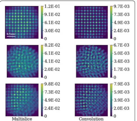
Figure 1 shows three examples of the convolution and multislice images produced from Pt nanoparticle models. The complete set of all images is provided in Additional file 2. The pixel intensity for the multislice simulations is normalized so that the total incident electron beam intensity is unity. The convolution simulations are scaled by the total integrated scattering cross section of the nanoparticle being modeled [33] which produces values typically about one order of magnitude less than the mul-tislice simulations. This scaling is used to bring the over-all convolution and multislice intensity scales into closer agreement, but is not essential to the quality of the fit.
The pixel intensity values in the images constitute the datasets used to create our models. Each image is roughly 250 × 250 pixels in dimension; so, each image contains roughly 62,500 pixels and each dataset of 18–20 images contains roughly 1.25 million convolution data points and 1.25 million corresponding multislice data points.
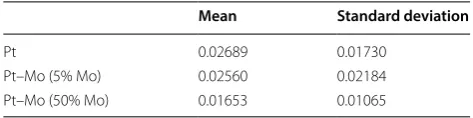
The means and standard deviations of our datasets are shown in Table 1. When calculating cross validation frac-tional root-mean-square error, we calculate the fraction of the standard deviation of the applicable data set [see Eq. (4)]; so, these values are used in many of the statistics given below.
Model assessment
We use cross validation to assess our models. We split our dataset into training and validation sets, fit the model using the training set, and use it to predict images in the validation set. We assign data to the validation and train-ing sets in three ways: by randomly assigntrain-ing images, randomly assigning 7 × 7 blocks of pixels, and randomly assigning individual pixels. We calculate cross valida-tion (CV) error by comparing the predicted intensity to the multislice intensity for each data point in the valida-tion set. This process is repeated a specified number of times with different validation sets. We report pixel-wise CV fractional root-mean-square (RMS) error and CV 1 −R2 error, where R2 is the coefficient of determination
between the predicted and multislice pixel intensities [34]. Results reported are computed in a single calcula-tion over all pixels in all cross validacalcula-tion sets.
Fractional RMS error ( EFRMS ) for a given predicted data set (which we will call the target set) is calculated as per Eq. 4, where n is the number of pixels in the
tar-get set, ypredi and yactuali are the predicted and multislice intensity values, respectively, of pixel i , ERMS is the root mean squared error, and yactual and σactual are the average
value and standard deviation of yactual over all pixels in the target set.
Results reported in the main text of this paper are for twofold cross validation with image-based subset assign-ment, repeated twice with different validation and train-ing subset assignments (i.e., 4 total validation data sets each of size 9–10 images, or 50% of our total data). For these two twofold cross validations on a full data set with N elements, the target set used in Eq. 4 would be two copies of all the N elements. A similar approach of using the full set of data across all left out groups as the target data to calculate standard deviations in Eq. (4) is used for other fractional CVs discussion in Additional file 1.
We chose to report the fractional RMS error as opposed to the raw RMS error as the intensities in the data being modeled have a complex normalization
(4) EFRMS=
ERMS=
i=n
i=1(ypredi−yactuali)2 n
σactual=
i=n i=1
yactual i−yactual
2
n
that makes it difficult to interpret the implications of the direct RMS. EFRMS is easy to interpret as a value of one is obtained for a model that simply returns the mean of the target set. Thus, values of significantly less than one suggest a model is meaningfully capturing the ways the target set is varying. In addition, we note that for our images, this quantity can be rewritten as EFRMS=ERMS/yactual/σactual/yactual . In this equation, the fraction in the numerator is the error normalized to the average intensity, and the fraction in the denominator is the contrast. Thus, EFRMS is also the ratio of the intensity normalized error to the contrast, which is a common way to consider the scale of errors in images.
In Additional file 1: Section S2.3, we show results of twofold cross validation for pixel-based and block-based subset assignments. In Additional file 1: Section S2.2, we show results of leave-out-X cross validation for selected values of X greater than 50% with image-based subset assignment to demonstrate model performance with training sets smaller than 10 images. These results are generally similar to those of image-wise twofold cross validation in the main text when the training set size is five images (~ 25% of our data) or larger. We also present plots of differences between predicted images and mul-tislice images for selected images in the main text, with additional images in Additional file 2.
All regressions and analysis reported in this work were performed in the Python 3 programming environment. Regressions were performed using the scikit-learn pack-age [35], version 0.18.1.
Timings given in this work are for the specific hardware used in this study. All regression and prediction calcula-tions were performed on hyperthreaded cores on CPUs of 2.1–2.7 GHz (20,000–30,000 million instructions per second). No parallelization was used.
Regression
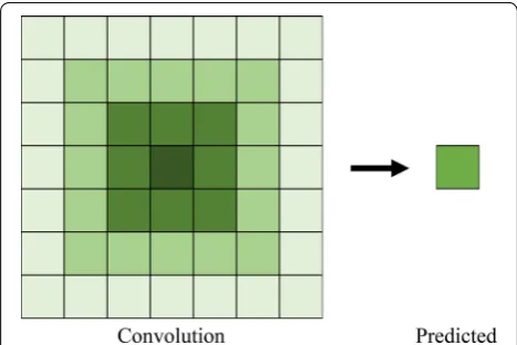
We performed multivariate polynomial regressions with the convolution image pixel intensities as the independ-ent variable and the multislice pixel intensities as the dependent variable. More precisely, for a given multislice pixel, the intensities of a group of pixels consisting of the corresponding convolution pixel and a number of sur-rounding pixels were used as input (see Fig. 2). We refer to this group of pixels as the input pixel grid. The fit is not location dependent. A single set of coefficients is learned for all possible inputs.
The input pixel grid size is defined by s , the grid side length measured in pixels. s must be an odd integer greater than or equal to 1. Pixels at the outer edges of the images could not be predicted in this way when s>1 due
to the lack of necessary nearest neighbors on one or two sides. We did not attempt to predict these edge pixels; so, Table 1 Summary statistics of multislice data
Mean Standard deviation
Pt 0.02689 0.01730
Pt–Mo (5% Mo) 0.02560 0.02184
the predicted images were cropped by s−1
2 pixels on all
sides.
The polynomials we tested vary in s , degree, inclu-sion of a logarithmic term, and incluinclu-sion of interaction terms. These variables are the adjustable parameters, or hyperparameters, of the regression model. Throughout this work, we use the word “term” to refer each element of the polynomial with a coefficient that is found via the fitting process. Hyperparameters were explored that create models with between 2 and 3654 terms, includ-ing the constant term. Additional file 1: Table S1 lists the hyperparameters and number of terms for each pol-ynomial tested.
Inclusion of a logarithmic term was tested to attempt to capture some of the different scaling of multislice and convolution intensity as atoms are added to a col-umn. Convolution intensity scales linearly as atoms are added to a column, while multislice intensity scales nonlinearly. Although a Taylor series can approximate a local logarithm when enough terms are included, we do not use polynomial terms of high enough order to ensure that they could adequately capture a logarithmic relationship.
We have not used any feature selection approaches (e.g., forward selection or principal component analy-sis) to reduce the number of descriptors. We felt that such selections could lead to removal of terms in ways that did not make physical sense. In particular, we assume that that the model should always include all powers up to the highest degree polynomial used as the behavior of the Y(X) function is fairly smooth and seems unlikely to actually be dominated by higher pow-ers without lower ones being present. However, this assumption is untested, and more exploration of ways to reduce the feature set is of interest for future work.
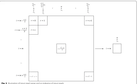
Figure 3 shows the input pixel grid required to esti-mate the intensity of a pixel with coordinates (m,n) . The side length of the input pixel grid is represented by s , which must be an odd integer greater than or equal to 1. Pixels in the grid have coordinates
i,j where:
For ease of reference, we re-index these pixel intensity values as xr , where
for a pixel with some set of coordinates
i,j
. The center pixel, with coordinates (m,n) , has index r=c= s2−1
2 .The general form of the polynomial can be written as
where
Here, we define the following variables: p=s2 is the total number of pixels in the input pixel grid, d is the
degree of the polynomial being fit, xp=log(xc) is an input term representing the logarithm of intensity of the center pixel, α=
0 if logarithmic term excluded
1 if logarithmic term included ,
β=
0 if interaction terms excluded
1 if interaction terms included , and akr , akp , akq ,
and a0 are regression coefficients. a0 is a constant term
and for the other coefficients the first index gives degree of the term being fit and the second index gives either the corresponding pixel [in Eq. (7)] or is the index of the term being fit [in Eq. (8)]. The first term in Eq. 7 is the single pixel intensity terms, excluding those due to the logarithmic input term. The second term is the single pixel intensity logarithmic terms. The third term, adapted from the expression for the complete homogenous symmetric polynomials [36], represents the interaction terms and involves all possible products of all included powers and logarithmic terms for all the pixel intensities.
(5) i∈m−s−1
2 ,m+s−21
, j∈n− s−1
2 ,n+s−21
(6) r=s
i−
m−s−1 2
+j−
n− s−1 2
= s
2
2 − s(i−m)+j−n− 1
2
(7) yc=
d
k=1 p−1
r=0
akrxrk+α d
k=1
akpxpk
+β d k=2 gk
x0,x1,. . .,xp
+a0
(8) gkx0,x1,. . .,xp=
b0+b1+ · · · +bp=k
0≤bi≤k−1
bp=0ifα=0
akqx0b0x
b1 1 . . .x
bp
p
Results and discussion Accuracy
As shown in Fig. 4, the accuracy of this approach is dependent on the number of terms included in the model. The best models yield a 1 −R2 twofold cross
vali-dation (CV) error of approximately 0.01–0.015, similar to that of relatively high-speed PRISM simulations [31]. The CV fractional RMS error of these same models is
approximately 0.1. CV fractional RMS error results for image-based twofold cross validation are reported in Additional file 1: Section S2.1. Error decreases sharply as the number of terms increases from two to approximately fifty. The marginal improvement gained per term added decreases significantly for models of above approximately fifty terms, and approaches zero for models above about 400 terms.
For models with more than approximately 200 terms, results for Pt, Pt–Mo 5%, and Pt–Mo 50% nanoparticles were similar. For models with less than 200 terms, results for Pt–Mo 50% were generally better than those for Pt and Pt–Mo 5%. The difference was particularly signifi-cant for models with less than 50 terms.
The number of terms is impacted by both polynomial degree and grid side length s. We assess convergence of errors with respect to each of these variables separately in Additional file 1: Sections S2.4 and S2.5 and find that s
values above 5 and polynomial degree above 3 confer lit-tle to no additional improvement in accuracy.
We take as optimal the model which appears to give the lowest CV 1 −R2 error within the general
uncer-tainty of the models while simultaneously using a few terms as possible. This model is a second-degree poly-nomial with s = 5, a logarithmic term, and all interac-tion terms (378 terms total). It is marked with a dashed Fig. 3 Illustration of input pixel range and re-indexing of input pixels
Fig. 4 Twofold cross validation 1 −R2 error as a function of
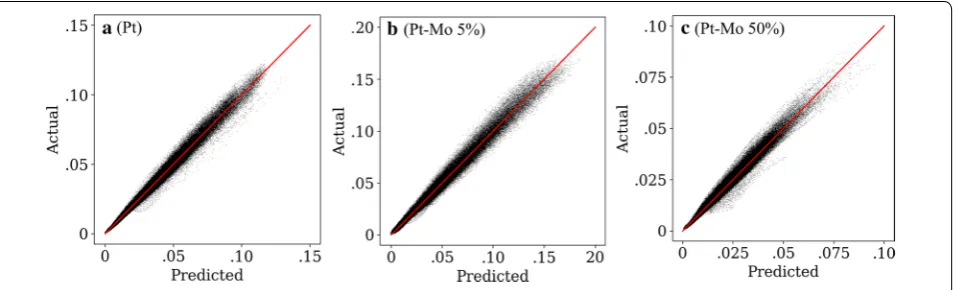
box in Fig. 4. This model would be a good choice for many applications, including the inverse structure determination problem addressed by Yu et al. Figure 5 shows pixel intensity parity plots (multislice pixel val-ues vs predicted pixel valval-ues) for this model. Parity plots for all other models tested can be found in Addi-tional file 2. The maximum intensity in the Pt–Mo 5% data is larger than that in the Pt data because the Pt– Mo nanoparticles were thicker than the Pt nanoparti-cles. The maximum intensity in the Pt–Mo 50% data is somewhat lower than in both the Pt and Pt–Mo (5% Mo) data because Mo has a lower scattering cross sec-tion than Pt. The CV 1 −R2 errors for these cases are
0.010, 0.012, and 0.014 for Pt, Pt–Mo 5%, and Pt–Mo 50%, respectively, demonstrating no large differences between compositions.
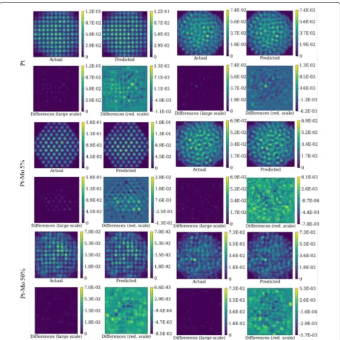
Figure 6 shows images of amorphous and crystalline Pt, Pt–Mo 5%, and Pt–Mo 50% nanoparticles created using the multislice method and the 378-term model. Two maps of the intensity differences between the pre-dicted and multislice images for each nanoparticle are also shown in Fig. 6: one on the same intensity scale as the multislice image and one on a reduced scale. Quali-tatively, the predicted images appear very similar to the corresponding multislice images and the difference plots on the scale of the original images look nearly uniform, indicating small errors compared to the over-all multislice intensity. The difference images do reflect the atomic structure, with the largest differences typi-cally occurring on the atomic columns. The on-column intensity has the strongest non-linear contribution from probe channeling and dynamical diffraction; so, this is perhaps an unsurprising result. Additional dif-ference plots for this model are included in Additional file 2. Figure S7 shows error as a function of pixel inten-sity for the 378-term model and confirms that generally,
error magnitude tends to be larger for higher-intensity pixels.
Speed
Once the training data set has been calculated using the multislice and convolution approaches, this STEM simu-lation method requires two steps: fitting and prediction. For each system of interest, the model must first be fit to a training dataset of convolution and corresponding mul-tislice images. This training dataset did not require very many images for the systems tested in this work. In the main text, we use a training set of nine–ten images to successfully simulate images of Pt and Pt–Mo nanopar-ticles of varying crystalline structures and topologies. In Additional file 1: Section S2.2, we use leave-out-X cross validation to show that training datasets as small as five pairs of images generally yield similar results. The com-putation time for the fitting step depends on the size of the training dataset and the number of terms in the model. It ranges between O(10−2) s (for a 2-term model
and 3-image training set) and O(104) s (for a 3654-term
model and 18-image training set) for the systems stud-ied here. The 378-term model, which Fig. 4 shows yields near-maximum accuracy, can be fitted to our nine- to ten-image training sets in O(102) seconds. This fitting
step need only be completed once per system.
Once the model is fit, the time taken to predict an image is negligible. For our structures and output image size (see “Methods” section) generating a convolu-tion image takes on order 10−2 s on one CPU. Applying
a model to a single point in a convolution image takes between O(10−9) s for a two-term model and O(10−6)
s for a 3654-term model on one CPU. As our images have approximately 62,500 points, applying the model to an entire convolution image therefore takes between O(10−5) s for a two-term model and O(10−2) s for a
3654-term model on one CPU. Thus, the application of the
models tested is comparable to or faster than the genera-tion of the convolugenera-tion image, and the total predicgenera-tion time of this approach for our structures is approximately five orders of magnitude faster than comparably accurate PRISM simulations [20].
Simple scaling arguments support that for models with O(103) terms or less, the application step will consistently
for the convolution image calculation scales in the same manner as the time for an FFT, or O(Nplog(Np)) with the
number of pixels in the image Np=Nx∗Ny , where Nx
is the x-dimension of the image in pixels and Ny is the y-dimension of the image in pixels. The convolution image calculation also scales linearly with the number of atoms in the system being modeled, Na . Time required for application of the model scales linearly with the num-ber of pixels in the image to which the model is applied and is independent of the number of atoms in the system. Thus, the ratio of the total time for applying a model to a convolution image over the time required to generate the convolution image scales as O(Nalog(Np)). Based on the
timings in this work, this ratio will be much greater than one for any reasonably sized system of even a few atoms or image of just a few pixels, and will clearly only increase for larger systems or images with more pixels.
Because the computation time for the convolution image generation step is comparable to or greater than the computation time for the model application step for models up to O(103) terms, the total prediction time for
this method will be approximately the same regardless of number of terms included in the model for models up to O(103) terms. However, larger models take more
time and memory to fit than smaller models, especially when the training set is large, and may be more prone to overfitting errors. In general, we strive to use the smallest model possible without sacrificing accuracy.
We emphasize that the method presented here is not a general method for calculating STEM images. The trained model is only valid in the domain of the training data. We have not explored the limits of applicability of our models beyond the training data set, but introducing new elements or new crystal structures that are not in the training data set is very likely to be beyond the validity of the model. It will always be better to train a new model for a new set of structures than to attempt to expand or adjust an existing model beyond its training data, espe-cially since only modest quantities of training data are required. We have also not explored the performance of this method for systems other than the three tested. It is likely that accuracy will differ for different materials and for systems containing different features, especially fea-tures that can modify the electron channeling behavior in the multislice simulation, such as interfaces. Exploring the limits of applicability of this method is an important task for future work.
Overall, this approach is best suited for applications where many images of similar structure and composi-tions (e.g, catalyst nanoparticles whose variation in com-position and morphology are well represented in the training set) must be simulated. In this case, the over-head time taken to generate a training dataset and fit the
model will be dominated by the time saved by significant speedup of many individual simulations.
Conclusion
We have presented a STEM image simulation method that combines a convolution of the probe point-spread function and the atomic potentials with a multivariate regression. The method involves generating a training data set of corresponding multislice and convolution images for a set of atomic models, then fitting a multi-variate function to predict the multislice result from the convolution result. After fitting to the system of interest, this method can be used to simulate images with approx-imately 0.01–0.015 twofold cross validation 1 −R2 error
and 0.1 twofold cross validation fractional root-mean-square error in just O(10−2 s/image) on a single 2.1–
2.7 GHz CPU. Once fitted, this method is several orders of magnitude faster than other STEM simulation tech-niques of comparable accuracy and is particularly use-ful for applications that require large numbers of image simulations of similar structures.
Additional file
Additional file 1: Table S1. Hyperparameters and number of terms for each polynomial tested. Table S2. Errors in individual cross validation folds, 2-fold cross validation with two repetitions, 378-term model. Figure S1. CV fractional RMS error as a function of number of terms in the regres-sion model for Pt and Pt-Mo nanoparticles. Results shown are those of image-based two-fold cross validation averaged over two repeats. Figure S2. CV error vs training set size for selected models. Leave-out-x cross validation used. Results are the average over 20 repetitions. (a), (d), (g), (j): Pt.(b), (e), (h), (k): Pt-Mo (5% Mo). (c), (f ), (i), (l): Pt-Mo (50% Mo). (a)-(c) and (g)-(i) present CV 1-R2 error. (d)-(f ) and (j)-(k) present CV fractional RMS error. (g)-(l) are presented on a set scale. Figure S3. Error for varying subset assignment schemes, selected models. (a)-(c): CV 1-R2 error. (d)-(f ): CV fractional RMS error. (a) and (d): Pt. (b) and (e): Pt-Mo 5%. (c) and (f ): Pt-Mo 50%. Figure S4. Two-fold CV error as a function of input grid side length (pixels) for models of constant degree, with a logarithmic term and without cross terms. (a)-(c): CV 1-R2 error. (d)-(f ): CV fractional RMS error. (a) and (d): Pt. (b) and (e): Pt-Mo 5%. (c) and (e): Pt-Mo 50%. Figure S5. CV error as a function of degree for models of constant input side grid length s (pixels), with logarithmic term and without cross terms. (a)-(c): CV 1-R2 error. (d)-(f ): CV fractional RMS error. (a) and (d): Pt. (b) and (e): Pt-Mo (5% Mo). (c) and (e): Pt-Mo (50% Mo). Figure S6. Cook’s distance for each point in a subset of each dataset, when fitted with the optimal 378-term model. (a): Pt. (b): Pt-Mo (5% Mo). (c): Pt-Mo (50% Mo). Figure S7. Error versus pixel intensity, 378 term model, two fold cross validation with two repeti-tions. (a): Pt. (b): Pt-Mo (5% Mo). (c): Pt-Mo (50% Mo).
Additional file 2. Training data, code, and additional results.
Abbreviations
Authors’ contributions
DM and PMV conceived the project. JJM, JF, and ZX generated multislice and convolution images for training datasets. AHC performed regressions and analysis of results. The manuscript was written by AHC with contributions from other authors. All authors read and approved the final manuscript.
Acknowledgements Not applicable.
Competing interests
The authors declare that they have no competing interests. PMV currently serves on the editorial board of the Springer-Open journal Advanced Structural and Chemical Imaging.
Availability of data and materials
All data and code used in this paper are included within its additional files. In addition, these materials are available on Figshare at https ://doi.org/10.6084/ m9.figsh are.74289 20.
Funding
We acknowledge the US Department of Energy, Basic Energy Sciences (DE-FG02-08ER46547) for support of this research.
Publisher’s Note
Springer Nature remains neutral with regard to jurisdictional claims in pub-lished maps and institutional affiliations.
Received: 10 May 2018 Accepted: 19 February 2019
References
1. Yankovich, A.B., et al.: Picometre-precision analysis of scanning transmis-sion electron microscopy images of platinum nanocatalysts. Nat. Com-mun. 5, 1–7 (2014)
2. Pelz, P.M., Qiu, W.X., Bücker, R., Kassier, G., Miller, R.J.D.: Low-dose cryo electron ptychography via non-convex Bayesian optimization. Sci. Rep. 7, 9883 (2017). https ://doi.org/10.1038/s4159 8-017-07488 -y
3. Yang, H., et al.: Simultaneous atomic-resolution electron ptychography and Z-contrast imaging of light and heavy elements in complex nano-structures. Nat. Commun. 7, 12532 (2016)
4. Miao, J., Ercius, P., Billinge, S.J.L.: Atomic electron tomography: 3D struc-tures without crystals. Science. 353, aaf2157 (2016)
5. Xu, R., et al.: Three-dimensional coordinates of individual atoms in materi-als revealed by electron tomography. Nat. Mater. 14, 1099–1103 (2015) 6. Scott, M.C., et al.: Electron tomography at 2.4-Å resolution. Nature. 483,
444–447 (2012)
7. Van den Broek, W., Rosenauer, A., Van Aert, S., Sijbers, J., Van Dyck, D.: A memory efficient method for fully three-dimensional object reconstruc-tion with HAADF STEM. Ultramicroscopy 141, 22–31 (2014)
8. Yang, Y., et al.: Deciphering chemical order/disorder and material proper-ties at the single-atom level. Nature 542, 75–79 (2017)
9. Johnson, J.M., Im, S., Windl, W., Hwang, J.: Three-dimensional imaging of individual point defects using selective detection angles in annular dark field scanning transmission electron microscopy. Ultramicroscopy 172, 17–29 (2017)
10. Zhang, J.Y., Hwang, J., Isaac, B.J., Stemmer, S.: Variable-angle high-angle annular dark-field imaging: application to three-dimensional dopant atom profiling. Sci. Rep. 5, 12419 (2015)
11. Kim, H., Zhang, J.Y., Raghavan, S., Stemmer, S.: Direct observation of Sr vacancies in SrTiO3 by quantitative scanning transmission electron
microscopy. Phys. Rev. X 6, 1–7 (2016)
12. Feng, J., Kvit, A.V., Zhang, C., Morgan, D., Voyles, P.M.: Bayesian statistical model for imaging of single La vacancies in LaMnO3. Microsc. Microanal.
23, 1572–1573 (2016)
13. Feng, J., Kvit, A.V., Zhang, C., Morgan, D., Voyles, P.M.: Three-dimensional imaging of single La vacancies in LaMnO3. Microsc. Microanal. 22,
902–903 (2016)
14. Kirkland, E.J.: Advanced computing in electron microscopy, 2nd edn. Springer, New York (2010)
15. Kirkland, E.J.: Computation in electron microscopy. Acta Crystallogr. Sect. A Found. Adv. 72, 1–27 (2016)
16. Allen, L.J., Findlay, S.D., Oxley, M.P., Rossouw, C.J.: Lattice-resolution con-trast from a focused coherent electron probe. Part I. Ultramicroscopy 96, 47–63 (2003)
17. Findlay, S.D., Allen, L.J., Oxley, M.P., Rossouw, C.J.: Lattice-resolution con-trast from a focused coherent electron probe. Part II. Ultramicroscopy 96, 65–81 (2003)
18. Cowley, J.M., Moodie, A.F.: Fourier images: I—the point source. Proc. Phys. Soc. Sect. B 70, 486 (1957)
19. Ishizuka, K.: A practical approach for STEM image simulation based on the FFT multislice method. Ultramicroscopy 90, 71–83 (2002)
20. Pryor, A., Ophus, C., Miao, J. A streaming multi-GPU implementation of image simulation algorithms for scanning transmission electron micros-copy. arXiv 1706.08563. 1–18 (2017)
21. Jones, L., Macarthur, K.E., Fauske, V.T., Van Helvoort, A.T.J., Nellist, P.D.: Rapid estimation of catalyst nanoparticle morphology and atomic-coordination by high-resolution Z-contrast electron microscopy. Nano Lett. 14, 6336–6341 (2014)
22. Yu, M., Yankovich, A.B., Kaczmarowski, A., Morgan, D., Voyles, P.M.: Integrated computational and experimental structure refinement for nanoparticles. ACS Nano 10, 4031–4038 (2016)
23. Xu, W., LeBeau, J.M.: A deep convolutional neural network to analyze posi-tion averaged convergent beam electron diffracposi-tion patterns. Ultrami-croscopy 188, 59–69 (2018)
24. Pizarro, J., et al.: Simulation of high angle annular dark field scanning transmission electron microscopy images of large nanostructures. Appl. Phys. Lett. 93, 153107 (2008)
25. Oelerich, J.O., et al.: STEMsalabim: a high-performance computing cluster friendly code for scanning transmission electron microscopy image simulations of thin specimens. Ultramicroscopy 177, 91–96 (2017) 26. Dwyer, C.: Simulation of scanning transmission electron microscope
images on desktop computers. Ultramicroscopy 110, 195–198 (2010) 27. Van den Broek, W., Jiang, X., Koch, C.T.: FDES, a GPU-based multislice
algorithm with increased efficiency of the computation of the projected potential. Ultramicroscopy 158, 89–97 (2015)
28. Hosokawa, F., Shinkawa, T., Arai, Y., Sannomiya, T.: Benchmark test of accelerated multi-slice simulation by GPGPU. Ultramicroscopy 158, 56–64 (2015)
29. Eggeman, A.S., London, A., Midgley, P.A.: Ultrafast electron diffraction pat-tern simulations using GPU technology. Applications to lattice vibrations. Ultramicroscopy 134, 44–47 (2013)
30. Yao, Y., Ge, B.H., Shen, X., Wang, Y.G., Yu, R.C.: STEM image simulation with hybrid CPU/GPU programming. Ultramicroscopy 166, 1–8 (2016) 31. Ophus, C.: A fast image simulation algorithm for scanning transmission
electron microscopy. Adv Struct Chem Imaging. 3, 13 (2017). https ://doi. org/10.1186/s4067 9-017-0046-1
32. Krivanek, O.L., et al.: Atom-by-atom structural and chemical analysis by annular dark-field electron microscopy. Nature 464, 571 (2010) 33. MacArthur, K.E., et al.: Probe integrated scattering cross sections in the
analysis of atomic resolution HAADF STEM images. Ultramicroscopy. 133, 109–119 (2013)
34. Olive, D.J.: Linear regression. Springer International Publishing, Berlin (2016). https ://doi.org/10.1007/978-0-387-45972 -1_5
35. Pedregosa, F., et al.: Scikit-learn: machine learning in Python. J. Mach. Learn. Res. 12, 2825–2830 (2011)