Efficient Computation in the Brain

(1)

University of Pennsylvania

ScholarlyCommons

Publicly Accessible Penn Dissertations

1-1-2015

Efficient Computation in the Brain

Xuexin Wei

University of Pennsylvania, [email protected]

Follow this and additional works at:http://repository.upenn.edu/edissertations

Part of theApplied Mathematics Commons,Neuroscience and Neurobiology Commons, and thePsychology Commons

This paper is posted at ScholarlyCommons.http://repository.upenn.edu/edissertations/2092

Recommended Citation

Wei, Xuexin, "Efficient Computation in the Brain" (2015).Publicly Accessible Penn Dissertations. 2092.

(2)

Efficient Computation in the Brain

Abstract

It has been long proposed that the brain should perform computation efficiently to increase the fitness of the organism. However, the validity of this prominent hypothesis remains debated. In this thesis, I investigate how this idea of efficient computation can guide us to understand the operational regimes underlying various cognitive functions, in particular perception and spatial cognition. In the first study, I demonstrate that such idea leads to a well-constrained yet powerful model framework for human perceptual behaviors by assuming the system is efficient both in term of encoding and decoding. This framework, when applying to human visual perception, explains many reported perceptual biases, including the repulsive biases away from prior peak, which are counter-intuitive according to the traditional Bayesian view. This framework also offers a principle way to address the common criticisms of Bayesian models in perception, which argue that Bayesian models are lack of constraints. In the second study, I demonstrate that the idea of efficiency, coupled with a few assumptions, allows us to make quantitative predictions on the functional architecture of the grid cell system in rodents. One such prediction is that the spatial scales of grid modules should follow a geometric progression, importantly, with the scaling factor to be close to the square root of transcendental number e ~1.6. Such zero-parameter predictions closely match the data reported in recent neurophysiological experiments. The theory also makes several other predictions, some of which have been confirmed by the data. This study suggests that achieving efficiency computation may also apply to neural circuits involving a high-level cognition, i.e. representation of space. In the third study, I analytically derive a generic connection between mutual information and Fisher information. This clarifies an important theoretical issue which has been misunderstood in previous neural coding literature. Additionally, it provides some powerful signatures of the Efficient coding hypothesis, which could guide future experimental tests. Together, the results presented in this thesis suggest that achieving efficient computation serves as a basic design principle which generalizes across neural systems processing low-level and high-level cognitive functions.

Degree Type

Dissertation

Degree Name

Doctor of Philosophy (PhD)

Graduate Group

Psychology

First Advisor

Alan A. Stocker

Second Advisor

Vijay Balasubramanian

Keywords

(3)

Subject Categories

(4)

EFFICIENT COMPUTATION IN THE BRAIN

Xue-Xin Wei

A DISSERTATION

in

Psychology

Presented to the Faculties of the University of Pennsylvania in Partial

Fulfillment of the Requirements for the Degree of Doctor of Philosophy

2015

Supervisor of Dissertation

Co-Supervisor of Dissertation

Alan Stocker

Vijay Balasubramanian

Assistant Professor of Psychology

Professor of Physics

Graduate Group Chairperson

John Trueswell, Professor of Psychology

Dissertation Committee:

David Brainard, Professor of Psychology

Russell Epstein, Professor of Psychology

(5)

Dedication

To my parents, Jun-Gang Wei and Xiu-Zhen Wei.

(6)

Acknowledgments

I would like to thank my advisors, Prof. Alan Stocker and Prof. Vijay Balasub-ramanian for their encouragement and support over the five-year Ph. D. period. Over time, I come to realize that Alan and Vijay differ in many ways in terms of the scientific style. However, there is one thing in common. That is to look for a simple and principled explanation underlying a set of seemingly diverse and complicated observations. I guess due to this reason, I often feel a sense of beauty and elegance in their science. I have benefited greatly from both of them.

I would like to thank Prof. David Brainard and Prof. Russell Epstein for their support throughout. As the Chair of my thesis committee, David always finds the easiest way to solve the problem every time I have a problem. Russell is always there for my random questions. I also want to thank the faculty members in the System Neuroscience group, including Prof. Josh Gold, Yale Cohen, Nicole Rust, Johannes Burge, Maria Geffen for various feedbacks on the materials presented in this thesis. Particularly, I acknowledge Josh for his valuable comments on Chapter 3 and another manuscript which is not included in this thesis, as well as spending time improving my talks.

I thank members in the CPC lab and the physics of living matter group for many interesting interactions. In particular, I want to thank Jason Prentice, for thinking about grid cells together these years. I am also especially grateful to Matjaz Jogan. He was almost always the first person listening to my stuff after I discovered something. I also want to acknowledge Pedro Ortega for sharing his knowledge about cybernetics and the ubiquitousness of rate-distortion theory. I thank Ann Hermundstad, who has kindly sent me her thesis as a template. I thank Alex Tank, Marcelo Mattar, Toni Saarela, Long Luu, Kristy Simmons, John Briguglio, Kamesh Krishnamurthy, Jan Homann for many fun conversations.

(7)

we did together in Peking University. I want to thank the folks in Penn Computa-tional Neuroscience journal clubs for every piece discussed together, including but not limited to Jeremy Manning, Yin Li, Marino Pegan, Drew Jaegle.

I want to thank all the people I met in the Cold Spring Harbor summer school in 2014. I had a wonderful experience there. In particular, I want to thank Bruno Ol-shausen, Greg DeAngelis, Greg Horwitz, Stefan Treue for the discussions on various work presented in this thesis. I want to thank Jonathan Pillow, Ann Churchland, Stephen Palmer, Geoffrey Boynton and others for many great games played to-gether.

I have been very lucky to meet and benefit from many great scientists outside UPenn during these years. The list is long so I shall not list it. Especially, I want to mention Prof. Eero Simoncelli, who always comes to my presentation in conferences. His constructive criticisms and insights have shaped this thesis in various ways. I also thank Eero for being an external member of my dissertation committee and for his careful reading of this thesis.

I am grateful to my family. My wife, Zi-Juan Chen, has always been supportive of me doing science, particularly during those difficult moments for me. Actually, if not for her, I probably would not ending up pursuing a Ph. D in UPenn. A substantial portion of the results presented here were obtained while sitting the train commuting to New Jersey, at the time when she was there. Special thanks to our dog, Small, who is now a three-year-old lovely Saint Barnard, for all the joy he brings to us.

(8)

ABSTRACT

EFFICIENT COMPUTATION IN THE BRAIN

Xue-Xin Wei

Alan Stocker

Vijay Balasubramanian

It has been long proposed that the brain should perform computation efficiently

to increase the fitness of the organism. However, the validity of this prominent

hypothesis remains debated. In this thesis, I investigate how this idea of efficient

computation can guide us to understand the operational regimes underlying

vari-ous cognitive functions, in particular perception and spatial cognition. In the first

study, I demonstrate that such idea leads to a well-constrained yet powerful model

framework for human perceptual behaviors by assuming the system isefficient both

in term of encoding and decoding. This framework, when applying to human visual

perception, explains many reported perceptual biases, including the repulsive

bi-ases away from prior peak, which are counter-intuitive according to the traditional

Bayesian view. This framework also offers a principle way to address the common

criticisms of Bayesian models in perception, which argue that Bayesian models are

lack of constraints. In the second study, I demonstrate that the idea of efficiency,

coupled with a few assumptions, allows us to make quantitative predictions on the

(9)

that the spatial scales of grid modules should follow a geometric progression,

im-portantly, with the scaling factor to be close to the square root of transcendental

number e _∼1.6. Such zero-parameter predictions closely match the data reported

in recent neurophysiological experiments. The theory also makes several other

pre-dictions, some of which have been confirmed by the data. This study suggests that

achieving efficiency computation may also apply to neural circuits involving a

high-level cognition, i.e. representation of space. In the third study, I analytically derive

a generic connection between mutual information and Fisher information. This

clarifies an important theoretical issue which has been misunderstood in previous

neural coding literature. Additionally, it provides some powerful signatures of the

Efficient coding hypothesis, which could guide future experimental tests. Together,

the results presented in this thesis suggest that achieving efficient computation

serves as a basic design principle which generalizes across neural systems processing

(10)

List of Figures

3.1 Bayesian observer model constrained by Efficient coding. . . 34

3.2 Prediction 1: Bayesian perception can be biased away from the prior peak. . . 38

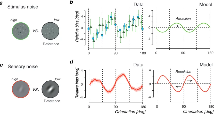
3.3 Prediction 2: Stimulus (external) and sensory (internal) noise dif-ferentially affect perceptual bias. . . 40

3.4 Biases in perceived orientation. . . 42

3.5 Relative biases in perceived orientation. . . 44

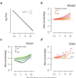
3.6 Biases in perceived spatial frequency. . . 47

3.7 Predicted biases for different loss functions.. . . 49

3.8 Equivalent efficient neural representations for the same stimulus dis-tribution. . . 55

4.1 Representing place in the grid system. . . 71

4.2 Optimal scaling factor of the grid system. . . 76

4.3 Dealing with two dimensional grid. . . 83

(14)

4.5 Optimizing the one dimensional grid system. . . 109

4.6 Encoding range can exceeds the period of the largest grid module. . . 118

4.7 The effect of lesioning grid modules on the distribution over location

for hierarchical vs. non-hierarchical grid schemes. . . 119

4.8 The effect of lesioning individual grid modules on place cell activity

in a simple grid-place transformation model. . . 121

5.1 Fisher information generally overestimates mutual information. . . 136

5.2 Different population tuning solutions lead to equivalent distributions

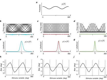
of Fisher information. . . 142

(15)

Chapter 1 Introduction

The human brain is a complex system which has attracted much endeavor to

under-stand how it works. The scientific investigations have traditionally been dominated

by the experimental approach, e.g. experimental psychology and neuroscience. In

such experiments, one typically manipulates a single variable at a time. By

observ-ing how the target variable changes, one could potentially obtain some

understand-ing about the underlyunderstand-ing process. Although a great deal of the knowledge about the

brain has been accumulated by this approach, one limitation is that it falls short

when dealing with the huge dimensionality of the underlying parameter space, and

when facing the complexity of computational machinery in the brain.

Starting from mid-20th century, scientists have gradually realized that, to

un-derstand the computations which gives rise to the various kinds of functions of the

(16)

use of mathematics and physics has many advantages and I shall only list a few

of them. First, such language makes it possible to precisely describing the process

of information processing in the neural systems. Second, one may gain some

fur-ther insights of such process by analytical investigations based on the formulated

mathematical model. Such insights, including these which may first appear to be

counter-intuitive, are otherwise difficult to obtain by, e.g. reasoning via human

language. Third, it could generate quantitative predictions to guide further

exper-imental investigation, and increase the chance of observing interesting phenomena.

The use of mathematics in neuroscience has already enjoyed some remarkable

suc-cess back to several decades ago, such as the landmark results of Hodgkin-Huxley

equations[93].

The approach of studying the brain by exploiting knowledge from mathematics

and physics have now lead to the field ofcomputational neuroscience [48]. Now there

seems to be an increasing agreement in term of that coupling the computational

approach with experimental approach offers the best promise to understand the

brain. Most existing work in the field of computational neuroscience deals with

computational models, which partly follows the tradition and style of the seminal

work of Hodgkin-Huxley equations [93]. Arguably, only a small portion of the

field deals with theories of the neural processing. Although the distinction between

theory and model is often considered to be fuzzy, I believe that the difference is real.

(17)

and model is that “(...) models describe a particular phenomenon or process, and

theories deal with a larger range of issues and identify general organizing principles”

[166]. While computational models are useful in providing quantitative descriptions

of the underlying biological process, they only shed limited general insight into the

designing principles of the brain. Overall, the computational modeling approach

often addressed the “how” question. However, a more comprehensive understanding

of the brain also requires asking the “why” question, which is typically the main

focus of theories in neuroscience.

Theories in neuroscience, although so far less well developed, have nonetheless

helped advanced our understanding of the brain in many ways. Notably, there

have been two lines of theoretical investigations which have substantial impact on

understanding of functions the brain, particularly perception. The first line of

theories promotes the idea of treating perception and cognitive functions in general

as an inference process, more specifically Bayesian inference(e.g. [103]). This route

could be traced back at least to Helmholtz (1866) [90]. In another line, neural

computation is formulated as a process of representing, recoding, and transmitting

information. Specifically, the Efficient Coding hypothesis by Attneave (1954) and

Barlow(1961) [10, 4] has sparkled a lot of following up investigations on early sensory

processing.

The research presented in the thesis is mainly driven by the theoretical approach.

(18)

otherwise appear to be unrelated, and the ability to predict what would be observed

in different situations. To this end, I have tried to test the developed theories using a

wide range of data, ranging from psychophysical measurements of human behaviors

to the neurophysiological measurements of neural populations in rodents.

1.1 Main hypothesis

The main hypothesis pursued in this thesis is thatthe brain performs computations

efficiently.

Various considerations jointly point to the concept that the computation in the

brain should be efficient (e.g. [113, 35, 112, 16, 116]). First of all, the computations

performed in the brain is costly in terms of energy. One remarkable observation is

that the brain, which typically consists 2% of the mass of the body, consumes 20%

of the resting metabolic energy [35]. Every spike and every synaptic event in the

brain requires energy [112, 116]. Second, consider the large variety of tasks which

the human brain can perform. These range from perception, navigation, identifying

objects, finding partners to solving math problems and thinking, writing. This is

particularly remarkable given the size and the limited amount of possible energy

consumption of the brain[112, 116]. To complete these various tasks successfully, the

brain has to somehow use the available information and energy efficiently. Third,

the survival pressure in evolution would tend to push the computations in the brain

(19)

pressure and limited resource (e.g. energy constraint, information constraint) faced

by the brain may have pushed the neural system toward the regime of being efficient

during evolution.

Historically, the concept ofefficiency has played an important rule in

formulat-ing theories of the brain computation. To appreciate this, let us briefly examine

these two influential lines of theories mentioned above. In the case of treating

per-ception as Bayesian inference, it could be seen as a result of couplingefficiency with

statistical estimation theory. While there are many possible ways of doing

statis-tical inference, the Bayesian inference representing the most efficient one. When

efficiency is coupled with Information theory [153], the Efficient Coding hypothesis

emerges [10, 4]. The appearance of the same concept in these two major branch

of theories should not be considered as surprising, given that efficiency provides a

fundamental, yet biologically well-grounded ingredient when formulating theories

of the brain computation.

In this thesis, building upon previous research, I test this main hypothesis in

both low-level and high-level cognitive functions of the brain, focusing on visual

perception and spatial navigation. I shall demonstrate that the idea that the brain

performs computation efficiently can explain a wide range of experimental

obser-vations, both in terms behavioral and neural measurements. Furthermore, it may

(20)

1.2 Structure of the thesis

In Chapter 1, I elaborate the concept of efficiency and why it may be relevant

for understanding the computations in the brain.

Chapter 2 aims to prepare the readers a minimal background for the materials

presented in the three following chapters, without thorough reviews of these

top-ics. In more details, it introduces i) two prominent hypothesis for understanding

perception, namely Efficient coding and Bayesian inference; ii) the basics of the

neurophysiological underpinning of spatial representation in rodent’s brain; iii) a

quick primer on Information-theoretic quantities, including the basic properties of

mutual information and Fisher information.

Chapter 3 develops a general framework for understanding perception. While

previous works on perception have either focus on the encoding or the decoding

as-pects, the presented framework integrates the idea ofEfficient coding andBayesian

decoding into a model of perceptual behaviors. I shall demonstrate that this

frame-work naturally accounts for various puzzling psychophysical observations reported

previously. The examples involved are from visual perception. This Chapter is

large part identical to a manuscript which has been submitted for consideration of

publication.

Chapter 4 applies the idea of Efficient coding to a high cognitive function, i.e.

neural coding of animal’s self-location during spatial navigation. Although

(21)

principle for understanding early sensory processing, however, it is largely unknown

whether such principle would also be relevant when studying high level cognitive

functions. In this chapter, I demonstrate that the notion of “efficiency”quantitatively

predicts the neurophysiologically observed functional architecture of the rodents’

grid cells, which form an representation of the space. This Chapter is large part

identical to a manuscript which has been submitted for consideration of publication.

In Chapter 5, I develop some analytically tools which clarifies the relationship

between mutual information and Fisher information - two widely used quantities

in neural coding. This important relationship has been misunderstood in previous

works. Furthermore, the results provide some powerful tests of Efficient coding for

future experiments. This Chapter is large part identical to a manuscript which has

been submitted for consideration of publication.

The final Chapter summarizes the contribution of the thesis, discusses open

questions and future directions which are likely to be fruitful.

Chapter 2 Background

Due to interdisciplinary nature of the research presented in this thesis, a brief

introduction for each topic seems to be desirable. In broad stroke, the research

are related to four different areas – Efficient coding, Bayesian inference, spatial

cognition, Information theory. Below I shall present the basics of each topic, with

the goal to facilitate the readers’ understanding of the following Chapters. Readers

who are already familiar with these topics should feel free to skip some of these

sections.

2.1 Efficient coding

One important hypothesis which drives the research on perception, in particular

early sensory procession, is the Efficient Coding Hypothesis. Efficient coding was

(24)

inspired by the seminal work of Shannon on information theory [153]. One key

con-tribution Atteave and Barlow brought into the field of neuroscience is the idea that

the mathematical framework of information theory may be relevant for

understand-ing the brain, and it may shed light on the strategy by which the neural system

process information.

Specifically, Barlow’s original version of Efficient coding concerns about how

information should be encoded in the sensory system, particularly in early visual

system. Barlow’s idea is that the sensory signal should be recoded in the most

economical way [10]. One particular way to increase efficiency, which is what Barlow

emphasized, is to make the response of the two outputs to be more independent,

i.e. redundancy reduction. The idea is simple. Redundancy between the output

units would lead to a decrease in terms of the information transmitted. Thus, if the

neural processing could somehow eliminate such redundancy, the efficiency of the

representation should be improved.

Many versions of Efficient coding theories were developed afterwards which

fol-low this idea of the efficient information transmission in the neural system. One

notable example is the proposal by Linker that the neural system should be

or-ganized in a way such that the mutual information between the input and output

should be maximized, i.e. InfoMax [121]. Importantly, Linsker also investigated

how biologically plausible learning rules might give rise to such efficient

(25)

One may wonder why there are many seemingly different versions of Efficient

coding theory co-existing in the literature. In my opinion, one reason is that

dif-ferent Efficient coding theories typically make difdif-ferent assumptions on the noise

structure of the system [154]. For example, in Barlow’s original proposal,

considera-tion of the neural noise is not included [10]. In this situaconsidera-tion, redundancy reducconsidera-tion

is a desirable goal. Linkser’s InfoMax could be related to the redundancy reduction

proposed by Barlow in the zero-noise limit. In some models, Gaussian noise are

assumed (e.g., [3, 179]). In the presence of certain type of noise, certain amount of

redundancy could actually be advantageous [3, 179, 55].

Another reason is that different theories may impose different constraints on the

overall resources and different objective functions. For instance, transmitting the

same amount information using the fewest number of spikes is, in general, a different

goal comparing to using the fewest number of neurons. These two objectives are also

different from the objective of using the smallest number of simultaneously active

neurons. These different assumptions would lead to different optimal configurations

of neural code. Interestingly, later work on sparse coding was inspired by

consider-ation of representing the input using a small number of active neurons [134, 135].

Some have argued that the optimal neural code should explicitly quantify and take

into account of the amount of energy consumption [119, 112, 7, 6, 116]. Some others

have argued that one should use the reconstruction error rather than the amount

(26)

Despite these different formulations, there seems to be one general agreement

among these theories, which is that the neural system should exploit the statistical

structure of the surrounding environment [63, 155]. This arises because,

funda-mentally, the amount of information transferred by a noisy channel, as well as the

reconstruction error, crucially depends on the probability distribution of the

in-put [153]. Because the inin-put to the sensory system will inevitably shaped (at least

partially) by the statistics of the environment, a good design of the sensory system

would have to take such statistical regularities into account.

Substantial efforts have been devoted to test the Efficient coding hypothesis

experimentally. Such investigations have lead to much success in early visual (e.g.

[111, 46, 6, 134, 59, 8, 100, 76]) and auditory processing (e.g., [120, 157]). However,

challenges remain. First, most studies have been done on early sensory system, and

it is presently unknown whether these results would generalize to relatively higher

cognitive area or not. Second, from a theoretical point of view, many previous

research have tried to predict the tuning property of individual neuron (e.g., [111,

127, 181]). However, arguably more desirable tests, which would shed more light

on the neural processing, should be tests at the neural population level. Third,

most previous work have focused on the predictions in terms of neurophysiological

(27)

2.2 Bayesian inference

Besides Efficient Coding, another major hypothesis which has profound impact on

the understanding of the perceptual process is the proposal of treating perception

as Bayesian inference (e.g. [103]). The basic idea is that perception is not simply

taking pictures of the environment like the way a camera does, rather it involves

active interpretation of the raw sensory inputs. Thus, perception could be better

viewed as an inference process. Holmherz already realized this concept in the 19th

century [90].

To appreciate the perspective of treating perception as an inference process [103],

it is useful to realize that there is virtually always ambiguity in the sensory input.

Consider the example of vision, in which 3-d environment is mapped to 2-d retinal

image. Some information becomes lost inevitably in such mapping. Also consider

the fact the noise is not only present in the stimulus itself, but it is also ubiquitous

along the sensory processing in the brain [60]. The presence of noise leads to

ambiguity when interpreting the sensory observation, and in principle could result

in many different interpretations of the same stimulus.

The noise in the perceptual process imposes a fundamental challenge for

per-ception (not only for visual perper-ception), namely, how does the perceptual system

select the specific way to interpret the input? An appealing hypothesis is that

per-ception involves efficient interpretation based on limited information gathered by

(28)

interpret the sensory observation.

Bayes’ rule

To understand how Bayesian inference works, consider the case of judging the

speed θ of an moving object. The perceptual system takes some observations of

speed of the moving object, which will be termed as “data”. Note that the process

which generates the data is typically noisy, in the sense that the mapping from a

particular speed θ to the data is not one-to-one, rather such dependence can be

summarized as a conditional probability distribution P(data_|θ). The problem is

that, once the data is known, how to infer the underlying speed of the object?

Bayesian inference tells us that one should use both the prior belief on the speed of

the moving object and the evidence gathered from the observations to perform the

inference. Furthermore, crucially one should combine these two source of

informa-tion using Bayes rule (Bayes &Price, 1763). Mathematically, Bayes’ rule could be

written as

P(θ_|data) = P(θ)P(data|θ)

P(data) (2.1)

This rule is the core of Bayesian inference. The term on the left-hand side

P(θ_|data) is the posterior distribution onθ given thedata. On the right-hand side,

P(θ) is typically referred as prior distribution onθ, which summarize the prior belief

(29)

of θ, which summarizes the evidence gathered from the data . It is important to

emphasize that although P(data_|θ) itself is a probability given θ, but with respect

to variable θ while fixing data, it is a function of θ, because its value varies with

θ. Therefore, it is appropriate to call it a likelihood function on θ, rather than a

“likelihood distribution”. Finally, the term P(data) is a normalization factor which

guarantees that P(θ_|data) is a proper probability distribution.

A common goal for Bayesian models is to derive the posterior distribution onθ,

i.e. P(θ_|data). This is, again, proportional to the product of the prior distribution

and the likelihood function. To get the posterior distribution, naturally one has to

obtain the prior belief and the likelihood function first.

To calculate the likelihood function precisely, in principle the full knowledge of

how the data are generated from θ is required. Such information critically depends

on the structure of the model (sometimes called “generative model” [48]). Of course,

the complexity of the problem varies depending on the structure of the model.

Chapter 3 has a detailed discussion on this issue, where I shall propose a principled

way to specify the likelihood function for certain perceptual inference problems.

How to specify the prior distribution? In practice, the selection of prior

dis-tributions is often done based on computation convenience. For example, a prior

distribution has often been chosen to be flat or Gaussian. Alternatively, a

seem-ingly more reasonable way is to pick up a “reference prior” [14] based on some

(30)

research topic in statistics [14, 101]. For perceptual inference, there may be

prin-cipled ways to specify the prior. Consider the speed example we mentioned again.

In this case, it seems reasonable to assume that such prior belief should depend on

our sensory experience in the past. This means that the prior distribution should

reflect the statistics of given variables in natural environments. Again consider the

example of the perceived speed. The prior may be thought as the statistics of the

speed in natural environments, which determines our long term sensory experience

on speed [169]. However, this is just a first-order approximation. In general, the

prior may depends on various other factors, e.g. context, individual, and so on.

Loss function

In many cases, computing the posterior distribution is not the end of the task,

because a particular Bayesian estimator may be required. For example, in the

con-text of speed estimation, a particular estimation of the speed of the object has to

be obtained, while the posterior distribution itself is not enough to specify the

per-cept. Technically, the mapping from the posterior to the Bayesian estimator could

be done by first assuming a loss function, and then constructing the corresponding

optimal estimator according to such loss [40]. Common choice of the loss functions

involves the family of Lp loss functions with pcan be chosen to be different values.

For squared error loss (p= 2), the resulting Bayesian estimator is the mean value

(31)

estimator is the median of the posterior distribution. The MAP estimator, i.e. the

mode of the posterior distribution, is obtained under 0₋1 loss (p = 0). Not too

much is known on the specific loss functions used by the perceptual system. We

will return to this point in Chapter 3.

2.3 Neural representation of physical space

As we navigate around, we often have a sense of where we are in space. Actually,

knowing the self-location relative to the environment is a fundamental ability for

the purpose of survival. How does the brain support such ability? Tolman (1948)

proposed that the brain should be able to maintain a “cognitive map” of the physical

space [174]. The discovery of place cells in rodent hippocampus around 1970s

has triggered a lot of following up research on the neural basis of spatial map in

the brain [132, 133]. The most salient property of place cells is that its firing

activity is sparse in space. Individual place cell typically fires when only animal is

within a particular spot in space [132], although some place cells fire in multiple

spots in space. As we know more about the place cells, it becomes clear that

the firing activities of the place cells are also correlated with many other factors

besides the animal’s spatial location, including odor, recent experience, time and

others [138, 2, 136]. The interpretations of these multi-perplexing responses are still

subjected to debates.

(32)

un-clear whether the spatial information is originated within hippocampus or inherent

from other brain areas. The discovery of grid cells in dorsal-medial Entorhinal

Cor-tex offers some new insight to this question[86, 75]. Now it appears that place cell

may, at least partially, inherent the spatial information from grid cells. Place cells,

grid cells, together with heading direction cells[172] and boarder cells[159] may

con-sist the neural underpinning of our sense of space during navigation. Studying the

properties and functions of these cell may provide us a unique chance to uncover

how the space is represented in the mammalian brain, and how spatial maps in the

brain support navigation behaviors, which are critical for the survival of mammals.

Grid cells

In 2004, Fyhn et al., discovered that in dorsal band of Entorhinal Cortex (EC)

of the rat’s brain, neurons typically show tuning preference for space, similar as the

place cells [75]. However, unlike place cells, these cells typically fire in the multiple

spatial locations. In 2005, a following up paper by Hafting et al., demonstrated that,

surprisingly, the spatial firing fields of the cells in dmEC lies on a triangular grid [86].

These cells are thus termed as “grid cells”. Because the highly regular firing pattern

of the grid cells, it is immediately suggested that the grid cells may encode a metric

of the space [86, 129]. Grid cells are also found in pre-and parasubiculum [19],

two brain regions next to EC. Although the response pattern of grid cells can be

(33)

which determines the response of the grid cells response appear to be the animal’s

location in space.

Why are grid cells not discovered in the studies before Hafting et al. (2005) [86]?

One major reason seems to be that previous experiments have used smaller testing

rooms, which were not enough to reveal the lattice structure of the grid. In a small

environment, typically only one or even zero firing field of individual grid cells could

be observed. However, in larger recording rooms, the pattern of the grid become

visually apparent. The grid is particularly evident when the two dimensional

au-tocorrelation map of the grid firing map is calculated which effectively reduce the

noise in the original firing rate map by averaging [86]. Originally found in rats, the

grid cells are later discovered in mice[74], and in bats [187]. There are some indirect

evidence from fMRI signal suggesting that grid cells may also exist in humans [54].

Recently, my colleagues and I have reported the first direct observation of grid-like

response in human brain by analyzing data from single neuron recording of human

epilepsy patients, while they were performing a virtual navigation task [94].

The response pattern of individual grid cell can be characterized by three

pa-rameters, the spacing, the orientation, and the spatial phase. Locally, the grid

cells in rodents share similar spacing and orientation [86, 164]. The spatial phase

seems to be shifted randomly such that nearby cells do not have nearby phases[86].

Therefore, there seems to be no topographical relationship in the spatial phase.

(34)

the grids. Furthermore, the scales increase systematically along the dorsal-ventral

axis [86, 26]. At the dorsal most, the spacing of the grid is about 50cm, while at

the 75% of the dorsal-ventral axis, the spacing of the grid can be several meters

to 10 meters, according to the recording when rats running on a 18 meters linear

track[26].

One particular important property of grid cells is that they are organized in

discrete structure [164]. By a fine sampling of grid cells along about half of the

dorsal-ventral axis of EC, Stensola et al. (2012) demonstrates that grid cells could

be clustered based on the scale, orientation and ellipticity [164]. The cells within

one cluster share the same scale, orientation and ellipticity. The individual cluster

is termed as a module. These authors found up to 5 modules within individual

animal. However, because the recording was only done up to 50% of the dorsal

ventral axis of EC, more modules should be expected in whole EC. A simple linear

extrapolation suggests that the number of the grid cell modules in rodent EC should

be _∼ 10. Strikingly, the data also suggest that the grid scales follow a geometric

progression. In this particular data set, the scaling factor was found to be _∼1.42,

while in a previous study, the scaling factor was reported be_∼1.7 with a relatively

smaller sample size [11].

The grid cells have attracted many computational investigations since it is

dis-covered. Most research have focus on the mechanisms and algorithms of how the

(35)

of pattern formation[176] in attractor network [72, 28, 20] and oscillatory

interfer-ence [30, 89], as well as spike rate adaptation [106].

While these computational models of grid cells aim to address thehow question,

the question of why the grid cells firing pattern should be as observed remain

mys-terious. In Chapter 4, I ask the fundamental issue in terms of why it is desirable

to use the grid code to form a representation of the space. I show that the idea of

efficient processing of spatial information quantitatively accounts for the functional

architecture of the grid cells observed in the rodent’s brain.

2.4 Mutual information and Fisher information

In this section, I introduce two important Information-theoretic quantities which

are used frequently in this thesis, namely mutual information and Fisher

informa-tion. Note that mutual information comes from Information theory, while Fisher

information has a fundamental root in statistics.

2.4.1 Mutual information

Information theory concerns the communication of information [153]. A basic

quan-tity in Information theory is entropy. Entropy characterizes the amount of

uncer-tainty associated with a random variable. For a discrete random variable X with

(36)

H[X] =Xp(x) lnp(x)

.

For a continuous random variableX with density p(x), its (differential) entropy

can be defined as

H[X] =

Z

X

p(x) lnp(x)dx

.

Mutual information quantifies how much information of one random variable

is contained in another random variable. Formally, mutual information could be

expressed as

I[X, Y] =H[X]₋H[X_|Y].

Note that following this definition, we can also consider

I[Y, X] =H[Y]₋H[Y_|X].

It can be verified that the following is true

I[X, Y] =I[Y, X].

For two continuous random variables X, Y, with joint probability densityp(x, y),

(37)

I[X, Y] =

Z

Y Z

X

p(x, y) ln

p(x, y) p(x)p(y)

dxdy.

Two important facts. First, I[X, Y] is always non-negative. Second, I[X, Y] = 0 is

equivalent to the independence of X and Y.

Information theory has profound influence in many scientific fields, including

neuroscience. In many neuroscience problems, one could treat individual neurons

or neural populations as noisy communication channel(s) and study the information

transmitted in such channel(s). For instance, denoting the stimulus variable as s,

and the neural response as r, one could compute the mutual information between

the stimulus and the response as

I[r, s] =H[r]₋H[r_|s].

This means that the mutual information is, technically, the difference between the

entropy of the response and the entropy of the response given a particular stimulus.

Conceptually, this captures the ratio between the volume of the response space and

the average volume of the response given a stimulus.

Alternatively, one could compute the mutual information as

(38)

computed as the difference between the entropy of the stimulus and the entropy of

the stimulus given a response. Conceptually, this is related to the ratio between the

volume of the stimulus and the average volume of the stimulus given a response.

Thus it quantifies how well a response r could tell about the stimuluss.

Recall the mathematical fact that I[s, r] is always identical to I[r, s], although

it should be apparent from the above discussions that the conceptual

interpreta-tions of these two quantities could be quite different. Practically, the mathematical

equivalence of these different expressions offers two choices for computing the

mu-tual information. Depending on the problems, one expression is usually easier to

work with compared to the other one. Unfortunately, sometimes both expressions

are difficult to compute exactly, in which cases one would need to rely on further

assumptions to work with these quantities.

2.4.2 Fisher information

Fisher information [67] is one central quantity in statistics, particularly in

estima-tion theory [115]. Fisher informaestima-tion is sometimes referred as “informaestima-tion” in

statistics [115]. Note that this should not be confused with mutual information

defined above. Fisher information characterizes the amount of information that

an observation (or measurement) m carries about an unknown parameter θ given

(39)

information can be defined as

J(θ) =

Z

∂lnp(m_|θ) ∂θ

2

p(m_|θ)dm. (2.2)

In this expression, p(m_|θ) should be treated as the likelihood function on θ.

lnp(m_|θ) represents the log-likelihood function, which is often called “support curve”[58].

The slope of the support curve is the “score”, which represents how sensitively the

likelihood function depends on the parameter θ. It is important to emphasize that

while the likelihood function depends on a particular observation m, Fisher

infor-mation does not. The reason is that the dependence on m is integrated out by

definition. Thus, it is appropriate to interpret Fisher information as a measure of

the expected sensitivity with respect to each value of the parameter θ, which is

fully determined by the encoding model which specifies the relationship between

the random variables m and θ. In some sense, Fisher information defines a metric

in the space of θ.

As a remark, there is another way to define Fisher information

J(θ) =₋

Z

∂2lnp(m_|θ)

∂θ2 p(m|θ)dm. (2.3)

It is straightforward to check that these two definitions are equivalent. These

defi-nitions only apply whenθ is a scalar. Ifθ is a vector, one can define a corresponding

(40)

Fisher information has many interesting properties. For the purpose of this

the-sis, I shall only introduce a few of them.

Cramer-Rao bound

Perhaps the most well-known result related to Fisher information is the

Cramer-Rao bound [41, 139]. Cramer-Cramer-Rao bound states that, under certain regularity

con-ditions, Fisher information sets an lower bound on the variance of any unbiased

estimator ˆθ. Formally, it could be expressed as

V ar(ˆθ)_≥ 1

J(θ). (2.4)

In general, Cramer-Rao bound could not be reached. It can only be tight for special

kinds of statistical models. I shall come back to this point later in Chapter 5, where

the conditions to make Cramer-Rao bound tight are discussed in some more details.

Intuitively, Cramer-Rao bound means that the quality of encoding, quantified by

the Fisher information, set a physical limit on how precise any unbiased estimator

can be.

Forbiased estimator, the corresponding Cramer-Rao bound turns out to be

V ar(ˆθ)_≥ [1 +b 0₍_θ_)]2

J(θ) , (2.5)

(41)

(mean square error) of estimator ˆθ must satisfy

M SE(ˆθ)_≥ [1 +b 0₍_θ_)]2

J(θ) +b(θ)

2_. _(2.6)

It is useful to point out that the MSE of a biased estimator could be smaller

than _J₍1_θ₎ which defines a lower bound for any unbiased estimator. Although many

might have the intuition that an unbiased estimator is advantageous compared to

a biased estimator, this result suggest that, counter to that intuition, having a bias

in the estimation could be actually desirable in certain situations.

Invariance of Fisher information

The square root of Fisher informationJ(θ) has a property of invariance, i.e.

p

J(θ)dθ =

q

J(˜θ)dθ,˜ (2.7)

where ˜θ is a re-parameterization of θ. As a corollary, the integral S =R pJ(θ)dθ

is invariant with respect to any re-parameterization of θ. Under these notations,

fJ(θ) = √

J(θ)

S behaves like a probability density. fJ(θ) is known famously as Jeffreys

prior [97], which is a widely used non-informative prior in Bayesian statistics [101].

As a remark, the integral R J(θ)p_dθ _{when taking} _p _{other than} 1

2 is not invariant

(42)

Relationship to psychophysical and neural measurements

Fisher information has widely applications in many scientific fields. In the

ex-treme, It has even been argued that Fisher information can provide a unification

of many area of science[71]. In this thesis, I shall focus on its possible applications

in terms of understanding the information processing in the brain. Let me start

by noting that Fisher information has a nice relationship with respect to the most

commonly taken psychophysical measurement, i.e. discrimination threshold. It has

been well-established that [152, 151] Fisher information sets an lower bound on the

discrimination threshold (_.θ) in fine discrimination tasks:

d(θ)_≥Cα

1

p J(θ),

whereCα is a constant determined by the specifics of the psychophysical procedure.

Fisher information can also be used to assess how much information a certain

neuron (or neurons) carries about a particular stimulus dimension. Consider a

Pois-son neuron with a smooth tuning curve f(θ). In this case, the Fisher information

has a nice close-form expression

J(θ) = Tf(θ)

02

f(θ) ,

where T represents the length of the integration time. There are several basic

(43)

curve of a Poisson neuron are important in terms of the Fisher information the

neuron’s response carries. Second, the neuron carries most Fisher information at

the flank of its tuning curve rather than the peak. Third, the Fisher information

scales linearly with the integration time and the gain of the neuron.

Fisher information and mutual information have intriguing relationships. On one

hand, by definition, Mutual Information and Fisher information are quite different.

Conceptually, Fisher information quantifies the local information, while mutual

information is a global measure. On the other hand, these two measures are also

(44)

Chapter 3 Bayesian observer model

constrained by Efficient coding

explains “anti-Bayesian percept”

3.1 Introduction

Perception involves two important stages of processing: 1) the representation of

incoming sensory information, and 2) the interpretation of that representation to

form a percept. Two prominent hypotheses have separately guided our

understand-ing of these two processunderstand-ing stages, but each has limitations when considered alone.

The Efficient Coding Hypothesis argues that neural resource limitations lead to

(45)

statistics of the natural environment [4, 10]. This hypothesis can explain several key

features of neural coding in early sensory areas (e.g.[134, 46, 120]), but it does not

specify how these coding characteristics can give rise to important aspects of

percep-tual behavior such as perceppercep-tual biases. In contrast, theBayesian Hypothesis posits

that perception is an act of unconscious inference that interprets the noisy sensory

representation in the context of prior knowledge about the world [90, 44, 103]. This

hypothesis provides a normative explanation for many aspects of perceptual and

sensorimotor behavior (e.g., [104, 169, 178, 98]), but it has been criticized for

us-ing arbitrary model specifications in order to explain psychophysical data [99, 21].

Here we unify ideas of Efficient coding and Bayesian inference into a new model of

perceptual behavior. Specifically, we propose an Bayesian observer model that is

constrained by assuming an efficient representation of the sensory input.

Two key components define a Bayesian observer: the prior belief that reflects the

observer’s expectation about how frequently a certain stimulus value occurs, and

the likelihood function that captures the encoding accuracy in the sensory

represen-tation of the observer. Previous studies have proposed independent constraints on

either the prior belief based on natural (e.g., [175, 83]) or learned (e.g., [96, 104])

stimulus statistics, or the likelihood function based on natural stimulus

uncertain-ties(e.g., [78, 29]) or neural physiological tuning characteristics (e.g., [169]), but

not both. In contrast, our new model formulation jointly constrains both the prior

(46)

well as the interpretation of the sensory evidence is optimized with regard to the

stimulus statistics of its sensory environment. Thus, we can specify a Bayesian

observer model for any stimulus variable with known natural statistics.

We validated our framework by formulating observer models for two perceptual

variables for which the natural statistics are known, visual orientation and spatial

frequency. The models make a number of distinct and rather surprising

predic-tions; e.g., that percepts are frequently biased away from the peaks of the prior, a

prediction that seems at odds with the standard Bayesian view. We demonstrate

that the predictions are well matched by data from several studies reporting

mea-sured biases in perceived visual orientation and spatial frequency under different

levels and sources of uncertainty. That includes biases that are seemingly

“anti-Bayesian” [23]. Our results demonstrate that by combining the ideas of Efficient

coding and Bayesian decoding, we can formulate well constrained observer models

that can account for perceptual behavior that has not been explained before. Some

earlier version of this work has been previously presented [184].

3.2 Results

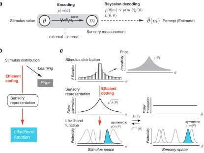
We model perception as a probabilistic encoding-decoding process (Fig. 3.1a) [169]:

The presentation of a stimulus with a single valueθ elicits a noisy sensory

measure-ment m (encoding), based on which the observer then generates an estimate ˆθ(m)

(47)

assumptions in order to define our observer model. First, we assume that

encod-ing is efficient, i.e., the sensory representation is optimally adapted to the natural

stimulus distribution. Second, we assume that decoding is Bayesian and is based

on an accurate (generative) model of the sensory process, i.e., the observer’s prior

belief matches the true stimulus distribution and the likelihood function faithfully

reflects the encoding characteristics. As a result, both the observer’s prior belief and

likelihood function are jointly constrained by the stimulus distribution (Fig. 3.1b).

Thus, with the additional assumption about the observer’s loss function (that states

how costly some perceptual errors are for the observer), we can make quantitative

predictions for the percept of a stimulus variable for which the natural stimulus

distribution is known. In the following we show how to formulate the model and

derive these predictions, and how they compare to measured psychophysical data.

3.2.1 Efficient coding and the likelihood function

We adopted a definition of Efficient coding that assumes that sensory encoding

maximizes the mutual information I[θ, m] between the sensory measurement m

and the stimulus variable θ with regard to the intrinsic uncertainty (internal noise)

in the sensory representation [121]. The definition establishes a link between the

(48)

Prior Probability Probability Stimulus space asymmetric c

Fisher Information

Likelihood function Prior Learning Efficient coding b Stimulus distribution # Samples Efficient coding Sensory representation Probability

Fisher Information

symmetric

Sensory space

a Encoding Bayesian decoding

Likelihood function Stimulus distribution Stimulus value Sensory measurement Percept (Estimate) Sensory representation internal external Noise

(49)

bound on mutual information [27, 127]. Assuming the bound is tight it follows that

p(θ)_∝pJ(θ) (see Methods for details). (3.1)

Fisher information J(θ) is a measure of encoding accuracy and reflects the amount

of sensory resources that is dedicated to the representation of a certain stimulus

valueθ. Equation (3.1) provides an intuitive way of understanding Efficient coding:

Sensory resources should be allocated according to the stimulus distribution p(θ)

resulting in a more accurate representation of those stimulus values that occur more

frequently.

Fisher information directly constrains the likelihood function, given our general

assumption that the likelihood function faithfully reflects the encoding

characteris-tics. But it is not sufficient to fully specify the shape of the likelihood function. An

additional assumption about the noise structure is required. Let us consider a

func-tion F(θ) that maps the stimulus space to a new space in which Fisher information

is uniform (see Fig. 3.1c). We refer to this space as the “sensory space” 1_{. With}

our chosen Efficient coding constraint Eq. (3.1) the mapping F(θ) is defined as the

cumulative of the stimulus distribution (prior) [111] (see Methods, Eq. (3.8)).

Uni-form Fisher inUni-formation implies that the noise and thus the likelihood function is

homogeneous. We introduce the additional assumption that the expected likelihood

1_{In reference to Gustav Fechner because discriminability, when measured in units of this space,}

(50)

function (i.e. averaged out over many trials) is symmetric around the stimulus value

in the sensory space. A simple way to guarantee this is to assume, for example, the

noise to be additive and symmetric (e.g. Gaussian as illustrated in Fig. 3.1c). For

a given sensory measurement m the likelihood function in the stimulus space can

then be obtained by simply applying the inverse mapping F−1(˜θ). As a result, the

likelihood functions when formulated in stimulus space are typically asymmetric

with a long tail away from the peak of the prior distribution.

Note that by formulating the Efficient coding in terms of Fisher information

we were able to specify the likelihood function without having to assume specific

details about the tuning characteristics of the underlying neural representation.

We deliberately chose such formulation because it allowed us a more parsimonious

yet also more general description of our Bayesian observer model. In fact, as we

demonstrate later, neural populations with quite different tuning characteristics

but equivalent distributions of Fisher information can represent equivalent efficient

sensory representations that lead to similar Bayesian decoding characteristics.

3.2.2 General predictions of the framework

The tight link between the stimulus distribution, the encoding accuracy (i.e., the

Fisher information J(θ)), and the shape of the likelihood function has important

consequences for the resulting decoding characteristics of our Bayesian observer

(51)

that are surprising and counter-intuitive from a standard Bayesian modeling point

of view.

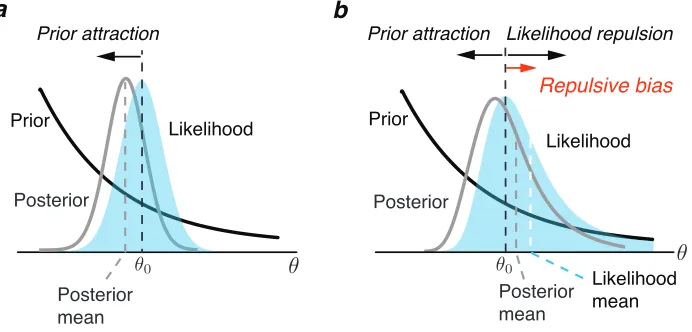
The first prediction concerns the effect of the likelihood asymmetry on perceptual

bias. A Bayesian modeling approach that assumes a symmetric likelihood function

predicts the percept to be biased towards the prior peak for relatively smooth prior

distributions (Fig. 3.2a). The situation changes, however, if the likelihood function

is asymmetric (Fig. 3.2b). Now, the asymmetry itself can lead to estimation biases

(see also [170]). In our framework, the shape of the likelihood is asymmetric for

any non-uniform stimulus distribution with a heavier tail pointing away from the

prior peak. This shape typically results in a repulsive bias component that we

refer to as the likelihood repulsion. Although the effect depends on the chosen loss

function, it is remarkably robust for commonly used choices (see Fig. 3.7). The

repulsive effect is further amplified when computing the expected bias over many

measurements of a given stimulus value θ0. The reason is that the distribution of

these measurements in the stimulus space also follows the same asymmetry; i.e.,

the noisy measurements and thus the position of the likelihood functions on each

trial are, on average, also biased away from the true stimulus value θ0. These

observations suggest a nuanced account of perceptual biases as the net result of

two bias components, one introduced by the likelihood asymmetry and one by the

prior distribution. Because of the above link, we can precisely predict the net bias

(52)

Posterior mean

Prior attraction Likelihood repulsion

Prior

Likelihood mean

Prior attraction

Prior _Likelihood

Posterior mean Posterior

b a

Posterior

Repulsive bias

Likelihood

Figure 3.2: Prediction 1: Bayesian perception can be biased away from the prior

peak. a) A standard Bayesian observer model that assumes a symmetric likelihood

function typically predicts perceptual biases toward the peak of the prior. This “bias towards the prior” has been considered a fundamental characteristic of a Bayesian model. b) In our new Bayesian observer model, Efficient encoding promotes a non-homogeneous sensory representation that leads to an asymmetric shape of the like-lihood function with a long tail pointing away from the prior peak. As a result, the estimate can be biased away from the prior peak. This is illustrated assum-ing the Bayesian estimate is determined by the posterior mean (squared-error loss function). Due to its asymmetry the mean of the likelihood function is away from the peak of the prior relative to the true stimulus value θ0 (Likelihood repulsion).

(53)

the model predicts that perception is biased away from the peak of the stimulus

distribution (i.e. the prior belief). In particular, assuming small sensory noise

only and a squared-error loss function (posterior mean) we can derive analytical

solutions for the expected perceptual bias for arbitrary stimulus distributions (see

Methods for details). The predicted bias is always repulsive if the prior distribution

is well approximated by a monotonic function over the support of the likelihood

function. This prediction is quite remarkable since the “bias towards the prior” has

been considered a fundamental characteristics of Bayesian observer models.

The second prediction is that stimulus (external) and sensory (internal) noise

differently affect perceptual bias. The difference emerges because our Efficient

cod-ing assumption generally imposes an inhomogeneous sensory representation that has

a different metric than the physical space. Thus, although ultimately both sources

of uncertainties are jointly reflected in the noise of the sensory measurementmtheir

individual effects on the likelihood function are different because of the mapping

functionF (Fig. 3.3a). As a result, the same noise added at the stimulus level leads

to a different likelihood function than the equivalent noise added at the sensory

level, which results in a different bias.

Increasing sensory noise results in a likelihood function that is more asymmetric

in the stimulus space because the additional uncertainty is mapped from the sensory

space (where it is symmetric; e.g. Gaussian) to the stimulus space via the inverse

(54)

a Perceptual bias + 0 Sensory noise repulsive attractive Stimulus noise - Prior Likelihood c Prior Prior Noise level Likelihood Likelihood low high low high more repulsion more attraction Stimulus space Stimulus space Sensory noise Stimulus noise Sensory space + + b

Figure 3.3: Prediction 2: Stimulus (external) and sensory (internal) noise

differen-tially affect perceptual bias. a) Stimulus noise directly affects stimulus uncertainty

(55)

likelihood function, the increase in likelihood repulsion generally dominates, leading

to a net increase in repulsive bias (Fig. 3.3b). Experimentally, we assume that

sensory noise (or rather the signal-to-noise ratio) can be modulated by changing

stimulus contrast or presentation time.

In summary, our Bayesian observer model predicts that perception is often

bi-ased away from the peak of the prior. Furthermore, it predicts that internal and

external noise can differentially modulate these biases: increasing internal noise

increases repulsive bias while increasing stimulus noise decreases repulsive bias,

eventually leading to attractive perceptual biases. These predictions are surprising

and at odds with predictions of standard Bayesian observer models.

3.2.3 Model validation against human psychophysical data

We validated the model predictions against measured perceptual biases for two

vi-sual stimulus variables with known natural stimulus distributions, local orientation

θ and spatial frequency ξ.

Orientation perception

Several studies have measured the distribution of visual orientations in natural

environments by carefully analyzing natural image data [37, 83]. The extracted

distributions are fairly robust with regard to the specifics of the analysis and the

(56)

Probability 0 0.01 Orientation [deg] 180 0 90 -10 0 10 Bias [deg] Orientation [deg] Noise Bias [deg]

@ 13.5 degs oblique

low high

Data d a b e c f low high Sensory noise -4 0 4 8 00 2 -2 0 Bias [deg] -4 4 high low Stimulus noise 0 3 -3 0 Model Model Data 180

0 90 0 90 180

180

0 90 0 90 180

Data

Orientation [deg]

-4

4

Figure 3.4: Biases in perceived orientation. a) Measured distribution of local visual orientation in natural images (gray line - re-plotted from [83]), superim-posed with the parametric description used for the model predictions (black line: p(θ) = c0(2− |sinθ|) where c0 is a normalization constant). b) Predicted mean

Efficient Computation in the Brain

University of Pennsylvania

ScholarlyCommons

Efficient Computation in the Brain

Xuexin Wei

Efficient Computation in the Brain

EFFICIENT COMPUTATION IN THE BRAIN

Xue-Xin Wei

A DISSERTATION

in

Psychology

Presented to the Faculties of the University of Pennsylvania in Partial

Fulfillment of the Requirements for the Degree of Doctor of Philosophy

2015

Supervisor of Dissertation

Co-Supervisor of Dissertation

Alan Stocker

Vijay Balasubramanian

Assistant Professor of Psychology

Professor of Physics

Graduate Group Chairperson

John Trueswell, Professor of Psychology

Dissertation Committee:

David Brainard, Professor of Psychology

Russell Epstein, Professor of Psychology

Dedication

Acknowledgments

Contents

List of Figures

Chapter 1

Introduction

1.1

Main hypothesis

1.2

Structure of the thesis

Chapter 2

Background

2.1

Efficient coding

2.2

Bayesian inference

2.3

Neural representation of physical space

2.4

Mutual information and Fisher information

2.4.1

Mutual information

2.4.2

Fisher information

Chapter 3

Bayesian observer model

constrained by Efficient coding

explains “anti-Bayesian percept”

3.1

Introduction

3.2

Results

3.2.1

Efficient coding and the likelihood function

3.2.2

General predictions of the framework

3.2.3

Model validation against human psychophysical data