Robust H
Control for A D.C Drive with
analysis of various performance measures
T.S. Viswanath1
Asst. Prof. Dept of IT REC, Bhalki
Karnataka India Dr. Subhash S.K2
Principal JPNCE, Mahabobnagar AP Abstract:
This paper presents the systematic robust controller design for d.c. drive. Based on a simplified model of the system. This drive system can accurately control and as good load disturbance rejection and tracking ability the paper uses loopshaping design to compute H controller using given optimization problem and specified weights the singular value plot of the sensitivity S , The complimentary sensitivity T and step response T are obtained
Key Words : H controller: robust control
1. Introduction
High starting torque, extended speed range, and ease of control in d.c. machines have ensured their continued use in industrial applications. Recent developments in d.c. machines usage have concentrated on drives using power semiconductor actuators (1). The most of the methods used for the design of controller are based on either conventional PID or Feedback / Feed forward compensator techniques. Applications of these methods have somewhat been restricted mainly due to the relatively slow speed of response and high capital cost of digital computers (2). In some cases the design employs techniques such as Bode, Nyquist plots and Nichols charts. However this method of design in trial and error but our approach completely eliminates the usage of Bode and Nyquist plots.
In addition to stability and enlarged stability margins. In this paper we have considered additional specifications of bandwidth, tracking, disturbance rejection, gainphase margins, compensator and plant bounds with internal stability constraint.
The paper is organized as follows. The problem statement is given in section II. Section III describes the design of robust controller for the given d.c. drive system. Illustrative example and results are given in section IV. Conclusions are given in section V.
2. Problem statement
It is desired to design a compensator for the given separately excited d.c. motor drive system such that the closed loop system tracks well at frequencies below wT = 0.4 rad / sec. with allowable error of 0.25 for step input,
has a bandwidth of WB = 1.1 rad / sec. (i.e. closed loop gain T (jw) = 0.707 for wwB) and has a gainphase
margins of m=1/2 with compensator and plant bounds of JC = 25 and w = 75 where,
CZ (jw) < = JC for all w and
Z (jw) < = w P-1 for all w.
The controller should also ensure internal stability of the sytsem 3. Design of robust controller
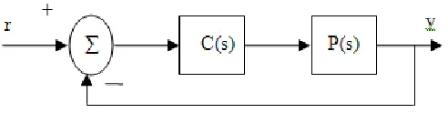
Fig. 1 Plant with controller
It desired to design a compensator C(s) for plant P(s) such that the closed loop system is internally stable and satisfies the desired performance measures as given in section II. For this system the sensitivity function Z(s) is defined as.
Z(s) = [1 + PC(s)]-1
(1) In frequency domain the sensitivity function is defined as Z(jw) = [1 + PC (jw)]-1
(2)
The first step is to convert all the requirements in terms of Z(jw), then the function Z(jw) is designed to satisfy these requirements. Once the requirements are satisfied then the compensator C(s) can be obtained from equation 1 as C(s) = P-1 (s) [Z-1(s) - 1] (3)
(1) Internal stability: The internal stability imposes the following constraints on Z(jw)[4]
Z ЄH ()
PZ ЄH <= => Z (0) = 0
[(Z-1-1)/P] Z=CZ Є H<= => Z () = 1 (4) and Lim S (Z(s)-1) = 0.
S
(2) Tracking error: Basically tracking error is time domain concept. In order to use frequency domain technique
one must translate time domain criteria back to frequency domain. The basic objective here is to make Z (jw) as small as possible particularly at low frequencies (wwT). Tracking error constraint is given as
ЄT = Sup Z (jw) (5)
wwT.
and is to be made as small as possible.
(3) Bandwidth: The main objective here is to ensure that the closed loop system is not upset by high frequency
noise. To satisfy this restriction, the gain of the system should be below the specified limit outside the bandwidth frequency wB. Thus the requirement is.
T (jw) <= for w > wB.
where = (T(jw) / T(0)
This imposes a constraint on z(jw) as
Z(jw) – 1 <= for w wB (6)
(4) Gainphase margin (m): the chief measures of robustness are given by gain and phase margins. Here we use a
composite measure of stability which seems at least as good. The composite measure of the gainphase margin can be defined as.
m = inf 1+PC(jw)
w
To have the required gainphase margin ‘m’ the constraint on Z(jw) is.
Z(jw) <= 1/m or all w (7)
(5) Compensator bound: In some cases the closed loop system will cause arcing at the output of the compensator
C(s) due to saturation. Therefore the compensator is to be bounded. For good compensation it is required that. CZ (jw) <= JC for all w.
for some prescribed number JC.
1 - Z(jw) <= JCP(jw) (8)
(6) Plant bound: In order to have the closed loop plant bounded by specified value w, the constraint on Z(jw) is.
Z(jw) <= wP(jw) -1 for all w
(9)
If the designed Z(jw) satisfies the equations (4) to (9), then the expression for the compensator C(s) can be obtained from equation (3).
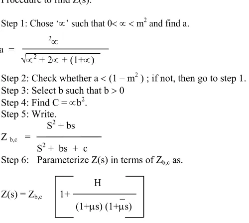
Procedure to find Z(s):
Step 1: Chose ‘’ such that 0 m2 and find a. 2
2 + 2 + (1+)
Step 2: Check whether a (1 – m2 ) ; if not, then go to step 1.
Step 3: Select b such that b 0 Step 4: Find C = b2.
Step 5: Write. S2 + bs
Z b,c =
S2 + bs + c
Step 6: Parameterize Z(s) in terms of Zb,c as.
H Z(s) = Zb,c 1+ _
(1+
s) (1+s)Where H is a rational function in H and is a scalar in R.H.P.
Step 7: Check whether Z(s) satisfies the equations (4). (9) ; if not satisfied goto step 3.
Step: 8: Obtain.
C(s) = P-1 (s) [Z-1(s)-1]
4. Illustrative example
In this section a solution is obtained for the problem stated in section II. First the mathematical model is obtained for the separately excited d.c. drive system and then the procedure outlined in section III is followed to design the robust controller.
4.1 Modeling: The figure 2 shows the functional block diagram of separately excited d.c. motor drive system (5)
Fig. 2: Functional block diagram of separately excited d.c. motor drives.
C(s) = (15)
Using thyristor based controller for motor armature voltage Ea (s), providing the inner current control loop to limit the armature current within some maximum allowable value, the modified block diagram of the separately excited d.c. motor drive system can be obtained as shown in fig. 2 (3).
figure
Fig. 3: Modified block diagram of d.c. motor drive.
Kic x Km2
(1+sjm )
Using the specifications of d.c. motor drive (3), the transfer function of the drive can be obtained as. 137.5
1+11.63s (12)
4.2 Design of compensator: In this subsection, the procedure outlined in section III is followed to design the
compensator C(s).
Taking =1/8 and b=8, the expression for Zb,c is
Zb,c = S2+8s
S2+8s+8
(13) Z(s) in terms of Zb,c is obtained as.
choosing H=1/(s+8) and =2, we get Z(s) as. 4s4 +36s3 +33s2 +9s
4s4 + 36s3 +65s2 +40s+1
(14) Substituting for P(s) and Z(s) in equation (3), we get. 372.16s3 +392.53s2 +124.04s +8
550s4 + 4950s3 +4537s2 +1237.5s.
4.3 Results: In this subsection the compensator C(s) as determined earlier, is tested to check whether all the
specifications and constraints are satisfied.
Internal stability: From relation (4) we get.
(16)
Z(0) = 0/8 = 0 Z () = 4/4 = 1
Lim s(Z(s)-1) = 32/ = 0
s
thus the controller satisfies all the internal stability constraints. and Kt = 1 (10)
Where P(s) =
P(s) =
TRACKING ERROR: Here Z(jw) is calculated for different values of w (for wwT) and the results are tabulated as shown
in
Table 1: Tracking error
w, in
rad / Sec Z (jw)
0.0 0.0 0.1 0.131 0.2 0.182 0.3 0.190 0.4 0.211 0.5 0.242
from the table it can be observed that tracking error Z(jw) is less than ЄT (here ЄT = 0.25) for w< wT (i.e., wT =
0.4), thus the system tracks well at low frequencies.
BANDWIDTH: To check the bandwidth constraint, Z(jw)-1 is calculated for different frequencies and results are
tabulated as shown.
Table 2: Band width
w, in
rad / Sec Z (jw)-1
0.0 1.0 0.1 0.991 0.15 0.983
0.2 0.97 0.4 0.91 0.8 0.79 1.0 0.737 1.1 0.707 1.2 0.67 2.0 0.48 10.0 0.06
from the table it can be observed that Z(jw)-1 is less than (here is 0.707) for w greater than 1.1 rad / sec., thus satisfying the bandwidth constraint.
COMPENSATOR BOUND: To check the compensator bound, 1-Z(jw) /P is calculated for different frequencies and the
results are tabulated as shown.
Table 3: Compensator Bound
w,
rad / Sec 1-Z (jw) / P
0 7.27e-3
1 0.0625 10 0.05
100 6.77e-3
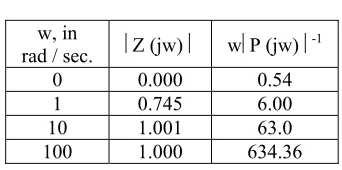
PLANT BOUND: To check for plant bound, Z(jw) is found out for different frequencies and results are tabulated as
shown.
Table 4: Plant Bond
w, in
rad / sec. Z (jw) wP (jw) -1 0 0.000 0.54 1 0.745 6.00 10 1.001 63.0 100 1.000 634.36
It is found that for all values of w Z(jw) <= wP (jw) for w=75, thus satisfying the plant bound.
GAIN PHASEMARGIN (M):To check the gainphase margin, Z(jw) is calculated for different frequencies and results are
tabulated as shown,
From the results it can be seen that for all frequencies Z(jw) is less than 2. Thus ensures the gainphase margin to be => ½. Thus the compensator also ensures the gainphase margin requirement.
Table 5 : Gain Phasemargin
w,
rad / Sec Z (jw)
0 0 1 0.745 10 1.001 100 1.00 1000 .
. . . .
1
Nomenclature
C(s) : Transfer function of controller Jc : Compensator bound.
Kic : Constant of current control loop.
Km2 : Gain of the motor constant (rad/sec)
Kt : Tachogenerator constant.
m : Gain phase margin. P(s) : Plant transfer function.
T(jw) : Closed loop gain in frequency domain. WT : Tracking frequency in rad / sec.
WB : Bandwidth frequency in rad / sec.
W : Plant bound.
Z (jw) : Sensitivity function in frequency domain. ET : Tracking error.
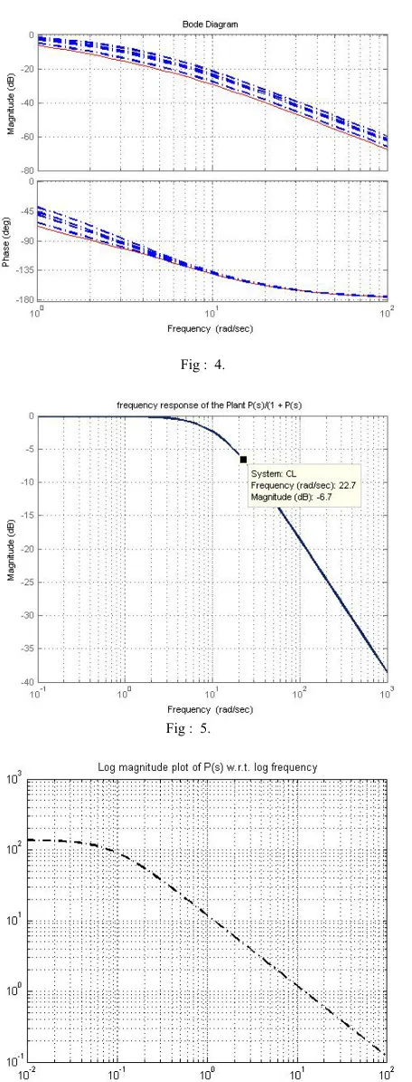
Simulation Results :
Fig : 4.
Fig : 5.
Fig : 7.
Fig : 8.
Fig : 10.
The Goal of the control design is to achieve the desired performance specifications on the plant model in the presence of model error and uncertainty the system has zero steady state error as shown in fig. (9) & (10) and tracks well at low frequencies as seen in the frequency response Plot shown in Fig. (1)
5. Conclusions
This paper proposes H controller design for a DC drive . The simulation results show that the whole drive system has good transient response, Load Disturbance response and Tracking ability in addition to achieving band width and bandwidth constraint. In this paper an attempt is made to design a new robust controller for separately excited DC. motor drive. It is found that with this controller, the system is internally stable; it rejects the high frequency, ensures the required gain phase margin and satisfies the compensator and plant bounds. However it is to be noted that the solution is not unique and that there is a serious trade off between bandwidth and tracking error which is evidenced by the fact that the reduction of bandwidth entails increase of tracking error in the d.c. motor drive system considered in this section. It is possible to reduce this error, simultaneously satisfying other specifications and constraints using the design freedom available. For any arbitrary set of specifications the existence of the solution is not guaranteed always. The paper gives existence and construction of the required compensator for multivariable system using Helton’s approach. The strength of this paper lies in satisfaction of number of practical requirements for d.c. drive system.
Acknowledgments
I am highly thankful to chairman to Sri. Eshwar Khandre & Principal Dr. B. B. Lal and my family members for there inspiration & help
References
[1] Robust Controller design for a Synchronous Reluctance Drive. IEEE transaction on Automatic control Vol II 1999,PP 809-814. [2] Controller design for a sensorless Permanent – Magnet Synchronous drive system. IEE proceedings-B Vol.140 No.6 1993 PP 316-374. [3] Hcontrol for a sensorless Permanent – Magnet Synchronous drive system IEE proceedings Electrical power applications Vol. 144 May
1997.
[4] Robust Control of DC Motor Using Fuzzy Sliding Control with PID Compemsator proceedings of the International Conference of engineers and Coputer Scientists 2009 Vol II March 18-20, 2009.
[5] R. John Hill and Fang L. Luo; “Microprocessor based control of steel rolling mill digital d.c. drives” IEEE transactions on Power Electronics, Vol. 4, No.2, April 1989, PP. 289-297.
[6] Jing-Oing Trang Shen Chen and P.K. Sinha; “Optimal feedback control of d.c. drives” IEEE transaction on Industrial Electronics, vol. 37, No.4, Aug. 1990, PP.269-274
[7] J. William Helton; “Worst case analysis in the frequency domain: The H approach to control” IEEE transactions on automatic control., vol.
AC-30, No. 12, Dec. 1985, PP. 1154-1170