The effect of various vertical discretization schemes and horizontal diffusion parameterization on the performance of a 3-D ocean model: the Black Sea case study

(1)

Ocean Sci., 9, 377–390, 2013 www.ocean-sci.net/9/377/2013/ doi:10.5194/os-9-377-2013

EGU Journal Logos (RGB)

Advances in

Geosciences

Open Access

Natural Hazards

and Earth System

Sciences

Open Access

Annales

Geophysicae

Open Access

Nonlinear Processes

in Geophysics

Open Access

Atmospheric

Chemistry

and Physics

Open Access

Atmospheric

Chemistry

and Physics

Open Access Discussions

Atmospheric

Measurement

Techniques

Open Access

Atmospheric

Measurement

Techniques

Biogeosciences

Open Access Open Access

Biogeosciences

Discussions

Climate

of the Past

Climate

of the Past

Discussions

Earth System

Dynamics

Earth System

Dynamics

Discussions

Geoscientific

Instrumentation

Methods and

Data Systems

Open Access

Geoscientific

Instrumentation

Methods and

Data Systems

Geoscientific

Model Development

Geoscientific

Model Development

Discussions

Hydrology and

Earth System

Sciences

Open Access

Hydrology and

Earth System

Sciences

Ocean Science

Discussions

Solid Earth

Discussions

The Cryosphere

Discussions

Natural Hazards

and Earth System

Sciences

Open Access

Discussions

The effect of various vertical discretization schemes and horizontal

diffusion parameterization on the performance of a 3-D ocean

model: the Black Sea case study

G. Shapiro1, M. Luneva2, J. Pickering1, and D. Storkey3

1_{University of Plymouth, School of Marine Science and Engineering, Drake Circus, Plymouth, PL4 8AA, UK} 2_{National Oceanography Centre Liverpool, Joseph Proudman Building, 6 Brownlow Street, Liverpool, L3 5DA, UK} 3_{Met Office, Fitzroy Road, Exeter, Devon, EX1 3PB ,UK}

Correspondence to: G. I. Shapiro ([email protected])

Received: 9 October 2012 – Published in Ocean Sci. Discuss.: 22 November 2012 Revised: 19 February 2013 – Accepted: 20 February 2013 – Published: 21 March 2013

Abstract. Results of a sensitivity study are presented from various configurations of the NEMO ocean model in the Black Sea. The standard choices of vertical discretization, viz.zlevels,scoordinates and envelopeds coordinates, all show their limitations in the areas of complex topography. Two new hybrid vertical coordinate schemes are presented: the “s-on-top-of-z” and its enveloped version. The hybrid grids usescoordinates or envelopedscoordinates in the up-per layer, from the sea surface to the depth of the shelf break, and z-coordinates are set below this level. The study is car-ried out for a number of idealised and real world settings. The hybrid schemes help reduce errors generated by the standard schemes in the areas of steep topography. Results of sensi-tivity tests with various horizontal diffusion formulations are used to identify the optimum value of Smagorinsky diffusiv-ity coefficient to best represent the mesoscale activdiffusiv-ity.

1 Introduction

The early ocean circulation models (Sarkisyan, 1962; Bryan, 1963) all usedzcoordinate vertical grids and a very coarse representation of the bottom topography. However, meteorol-ogists who started using numerical models a decade earlier (Charney et al., 1950) have found that using azcoordinate system has certain computational disadvantages in the areas of varying topography, in particular in the vicinity of moun-tains. To resolve this problem a terrain-following sigma-coordinate system was introduced (Philips, 1957). Similar

constraints on the use of zcoordinate have been found in ocean modelling (see e.g. Blumberg and Mellor, 1983) in particular where both the shelf seas and the deep ocean are included in the model domain. Thezlevel systems have a lower number of layers in the shallow than in the deep re-gions, which makes it difficult to resolve the water column properties equally well. The effects of vertical discretization on the bottom boundary layer dynamics were studied by Ezer and Mellor (2004) for the idealised case of plain bottom slope. In this paper we extend such analysis for real world bathymetry which combines gentle shelves and steep conti-nental slopes.

(2)

are widely used in modern numerical models, such as POM (Princeton Ocean Model) or POLCOMS (Proudman Oceanographic Laboratory community model system). How-ever the terrain-following grids have their own disadvantages due to the errors in calculation of the pressure gradient force (see e.g. Rousseau and Pham, 1971; Mellor et al., 1994; Ezer et al., 2002). The error is partly caused by violating the con-dition for “hydrostatic consistency” (Rousseau and Pham, 1971), which is often written in the form as follows:

|R|<1; R=σ×δxH

H×δσ , (1)

whereσ is the sigma coordinate of a numeric cell, H its depth below sea surface,δxH the change in depth of hori-zontally adjacent grid cells, andδσ the vertical grid size in sigma coordinates. On a sloping topography this condition is severely restrictive. Mellor et al. (1994) have shown that, when using fine vertical resolution, a numerical scheme can be hydrostatically consistent even whenR >1 as the trunca-tion error contributing to the “inconsistency error” is propor-tional to the following:

Err∼(δσ )21−R2 (2)

and can decrease with increasing vertical resolution. There were multiple attempts to introduce alternative or generalised vertical grid systems that would increase the ac-curacy of numerical calculations; some of them use vertical grids which are not geometrically fixed but evolve in time. Examples include adaptive vertical grids (see Hofmeister et al., 2010, and references therein), isopycnal models such as MICOM (see Bleck et al., 1992), and hybrid models that combine isopycnal, sigma andzcoordinate systems such as HYCOM (see Bleck, 2002). Each of these model types has its own advantages and disadvantages (see e.g. Hofmeister et al., 2010). However the most popular grids used in ocean modelling are based on traditional sigma andzlevel schemes or their combination and variants due to their computational efficiency.

Ezer and Mellor (2004) compared sigma andzlevel grid simulations in a highly idealised dense water flow down a sloping bottom. Thezlevel grid performed relatively poorly due to the step-like representation of topography. However increasing both the horizontal and vertical resolution in thez

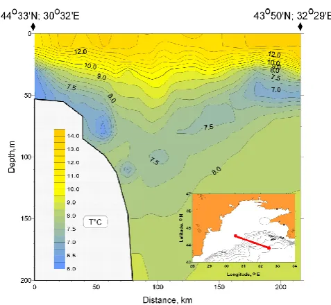
Fig. 1. Dense water cascade in the Black Sea, May 2004, (Shapiro, 2008).

level model converged results toward lower-resolution sigma grid (Legg et al., 2008). Mellor et al. (1994) demonstrated, in an idealised setting, that the model is stable and the spurious currents decrease with time even whenR=13 if the vertical resolution is sufficiently fine. The modelling of a near-bottom density current over a very steep (39>) slope using thes co-ordiante grid (a derivative of sigma) was stable and in a good agreement with laboratory experiments at R=101 subject to having 4–10slevels within the thin bottom plume (Wobus et al., 2011). The “safe” value ofRalso depends on the ac-tual topography and the numerical scheme (Shchepetkin and McWilliams, 2009), so sensitivity studies are required to test vertical discretization for specific model configurations.

(3)

G. Shapiro et al.: The effect of various vertical discretization schemes/horizontal diffusion parameterization 379

b

c d

a

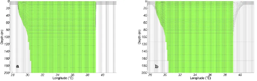
Fig. 2. Standard NEMO vertical grids shown at a Black Sea transect along 44◦N. Green areas represent wet points included in computations; white areas represent masked-out dry points. Dots show location of T-points within the cells. There is an extensive shelf on the western side of the transect and a very narrow shelf on the eastern part, which is not resolved by the model. (a)zcoordinate grid (ZCO); (b)scoordiante grid (SCO). The undulation of the numerical levels is due to the underwater ridge which is shallower than 1550 m; (c)scoordiante grid with enveloping topography (Z*SIG). For clarity, only the upper parts of the grids are shown in subfigures (a)–(c). The Z*SIG grid for the full depth of sea is shown in subfigure (d).

2 The grids

The NEMO-SHELF numerical model is a 3-D hydrostatic, baroclinic primitive equation model laid out horizontally on the Arakawa C-grid (Madec et al., 1998; NEMO, 2010; O’Dea et al., 2012). Five configurations of NEMO were generated for this study by utilising a number of vertical grids. These grids include 3 standard grids used in NEMO-SHELF:zlevel (ZCO), s coordiante (SCO) (see Song and Haidvogel, 1994),scoordiante with enveloping topography (Z*SIG, using designation from O’Dea et al., 2012) and two grids specifically developed for this study (Shapiro et al., 2012): the hybrid on-top-of-z” (SZH) and the hybrid “s-enveloped-on-top-of-z” (SZHENV). Bottom topography was derived from ETOPO2 database (ETOPO2v2, 2006). In or-der to suppress unnecessary curvature of terrain-following coordinates in the upper layer due to variations of bottom topography below 1550 m, the deepest numerical level (w level) was forced to be horizontal at this depth level to rep-resent an “artificial bottom”. It is a common view that the currents below 1000–1200 m are negligibly small (Demy-shev et al., 2002; Enriquez et al., 2005); so the waters be-tween 1550 m and the seabed were excluded from the

sim-ulation. The transition between the artificial and real bottom was slightly smoothed with a 9-point, 2-D filter. Another ad-vantage of such configuration is that, by reducing the depth of the sea, we can increase the barotropic time step in the time splitting scheme.

(4)

Fig. 3. Same as Fig. 2 for the new s–z hybrid grid (SZH) and the s–z hybrid enveloped grid (SZHENV).

The standard grids are shown in Fig. 2. The ZCO grid gen-erates serrated edges near the shelf break, exactly where the cold shelf waters sink to a greater depth in the spring sea-son. The SCO shown in Fig. 2b produces a smooth terrain-following grid. However, it violates the “hydrostatic con-sistency” condition in many places around the shelf break. While such a grid will not necessarily produce wrong results (see Mellor et al., 1994; Wobus et al., 2011), the results should be carefully analysed.

The improvement on the standard SCO grid is the s-grid with the enveloping topography (Z*SIG) (see NEMO, 2010). The generation of the enveloping topography starts from the deepest part of the sea and is calculated using the following criteria:

rn=max

henv_ij −henv_{i+1, j}

henv_ij +henv_{i+1, j} ,

henv_ij −henv_{i, j+1}

henv_ij +henv_{i, j+1} !

<rncr (3)

wherehenv_ij ,henv_{i+1, j}, andhenv_{i, j}₊₁are the depths of adjacent grid points in the enveloping topography. Based on common prac-tice the threshold is set to rncr=0.1.

The grid cells which are below the actual bottom are masked out in Fig. 2. The enveloping algorithm improves hydrostatic consistency. However, too many numerical lay-ers go below the bottom too early, hence reducing vertical resolution on the shelf and shelf break (see Fig. 2c–d). Such loss of vertical layers is caused by steep lower continental slopes and upper continental rise, where the currents are very small. Due to very weak stratification at these depths, the er-rors caused by not satisfying condition (2) are unlikely to be large, so that the loss of resolution in the Z*SIG grid is un-necessary.

In order to eliminate or reduce the loss of vertical resolu-tion common for the Z*SIG grids, combine the advantages of both ZCO and SCO grids, and minimise their disadvantages, a new hybrids–zcoordinate grid (SZH) has been introduced. This grid consists of a standard SCO in the upper part of the sea (in this case above 100 m) and ZCO grid below 100 m. This grid is shown in Fig. 3a. The vertical levels are hori-zontal over the majority of the basin and become curved to

follow topography only where necessary. Most places where the depth does not exceed 100 m, the shelf is sloping gently and the “hydrostatic consistency” condition (2) is satisfied even at relatively modest vertical resolution. However there are few places in the Black Sea where shelf is steep even if the depth is less than 100 m. To cater for such cases the SZHENV grid has been developed, which has the envelop-ing Z*SIG in the upper part of the sea and ZCO in the lower part (see Fig. 3b). There is a minimal loss of numerical levels (3 out of 18) in the shallowest grid cell in the western part of the transect.

It order to compare performance of various grids, we car-ried out a number of idealised simulations, for which the solution is known, some idealised cases where solution is known only approximately and real world simulations where the results are compared with satellite-derived sea surface temperature.

3 Idealised simulations

The first set of idealised simulations used the initial con-ditions produced by spreading horizontally a real temper-ature/salinity profile, obtained from a climatic atlas of the Black Sea for the month of January (Suvorov et al., 2004). There was no forcing either via meteorological fields, rivers or exchanges via Bosporus. In such conditions there should be neither currents nor a change in temperature and salin-ity, except a very small, horizontally homogeneous, verti-cal diffusion due to background diffusivity. However, due to computational errors, the spurious currents develop over time. Temperature stratification also becomes horizontally non-homogeneous. Results of simulation after 3.5 months are shown in Figs. 4 and 5.

(5)

G. Shapiro et al.: The effect of various vertical discretization schemes/horizontal diffusion parameterization 381

Fig. 4. Spurious zonal velocities along 31◦E after 3.5 months of simulation: (a) ZCO; (b) SCO; (c) Z*SIG; (d) SZH; (e) SZHENV.

SZHENV; they are unacceptably high for SCO and Z*SIG. The currents result from spurious density gradients generated by uneven numerical diffusion of temperature and salinity (see Fig. 5). The spurious gradients in ZCO-coordinates seem to come from the bottom boundary condition in the GLS turbulent closure scheme, which generates increased vertical diffusion near bottom due to insufficient vertical resolution.

The second set of idealised simulations was carried out for the initial conditions consisting of a conical inter-face with a horizontal brim (see Fig. 6f). The temperature above and below the frontal interface was set at 15◦C and 10◦C, respectively; a constant salinity of 18 psu was ap-plied throughout the basin. This setting mimics the dome-like structure of the pycnocline in the Black Sea. The frontal interface has a constant slope, and, according to the “thermal wind” equation, the difference between horizontal velocities

above and below the interface must not change horizontally. In this setting thezcoordinate (ZCO) grid loses its a priori advantage of the numerical levels being parallel to the isopy-cnals as it was in the first set of simulations.

Figure 6 shows that the best uniformity of the velocity field and minimal spurious currents are generated by the ZCO grid. The Z*SIG and SZHENV produce similar results with very small spurious velocities. The standards coordiante is the worst; the SZH grid also produces, however to a lesser extent, spurious currents near the steep continental slope.

4 Black Sea circulation

(6)

(7)

Fig. 6. Zonal velocity distribution along 43.3◦N after 1 month of simulation of the conical front: (a) ZCO; (b) SCO; (c) Z*SIG; (d) SZH; (e) SZHENV. (f) initial temperature transect is shown only for ZCO; other configurations are very similar.

temperature and salinity from the Black Sea atlas (Suvorov, 2004) were interpolated onto the model grids. Then short convective adjustment runs were invoked for a few time steps with very high vertical diffusivity (100 m2s−1) to eliminate small density inversions due to interpolation. Then the model was spun-up for about 7 months with no meteorological forc-ing and river discharges followforc-ing the procedure detailed in Enriquez et al. (2005), i.e. by freezing initial temperature and salinity distributions and allowing the currents to achieve an equilibrium with the density field.

The main simulations were driven by meteorological forc-ing from the SKIRON forecastforc-ing system (http://forecast. uoa.gr/index.php) with 10×10 km resolution using the CORE formulation (see Large and Yeager, 2004). The

(8)

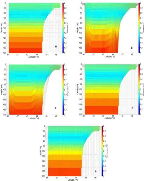
Fig. 7. Temperature transects along 31◦E for 16 April 2007: (a) ZCO; (b) SCO; (c) Z*SIG; (d) SZH; (e) SZHENV.

For the analysis we selected the transect along 31◦E. Whilst we do not have observational data (the “truth”) on this transect due to lack of observation, the model skill can be assessed qualitatively by comparing model results with typical partial transects and individualT /S profiles obtain-able from the Black Sea databases (Suvorov, 2004). Such an approach allows us to identify significant deviation of the model from typical observations. Temperature cross-sections for 16 April 2007 are shown in Fig. 7. As expected, the z-grid has coarser vertical resolution at the location of the cold wa-ter plume penetrating from the shelf into the cold inwa-terme- interme-diate layer as compared to the terrain-following grids. This results in a “broken” plume and disappearance of bottom cold water on the shelf. Insufficient resolution could also lead to errors in estimating the downslope velocities of the

near-bottom plume (Legg et al., 2008; Wobus et al., 2011) and hence the efficiency of the CIL replenishment. However the z-grid conserves well the CIL in the deep part of the sea. The sigma-grids, both SCO and Z*SIG, generate a reason-able representation of the cold water plume. However, it is “broken” on Z*SIG grid, probably due to high and patchy spurious velocities (see Fig. 7). The SCO grid does not con-serve well the CIL in the open sea. The hybrid grids, SZH and SZHENV, preserve well both the cold plume at the shelf break and the CIL in the open sea, with SZH doing its job slightly better.

(9)

Generation of unrealistic currents by SCO and Z*SIG is con-sistent with generation of large spurious currents by these grids in the first idealised test. The ZCO, SZH and SZHENV grids produce more realistic results which are generally con-sistent with those reported in the literature (Stanev et al., 1998; Demyshev et al., 2002; Zatsepin et al., 2003; Shapiro, 2008).

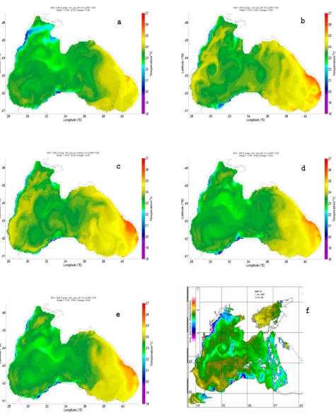
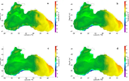
The ability of the model with different grids to repro-duce realistic sea surface temperature (SST) is examined in Fig. 8 where model results are compared with SST charts obtained from the Remote Sensing Department of the Ma-rine Hydrophysical Institute (dvs.net.ua). As in the previous test, the model was initialised with climatic initial conditions and ran from 1 January to 7 July 2007 without data assimi-lation. The main feature seen in the satellite image is a cold water filament spreading from the tip of the Crimean penin-sula to the SW corner of the sea and an intensive anticyclonic eddy containing cooler waters of about 23◦_{C (see Fig. 8f).} These features are best represented by ZCO grid, and reason-ably well by SZHENV. The standard sigma grids, SCO and Z*SIG, misplace the eddy and produce significant warmer ar-eas along the western coast which are not seen on the satellite SST image.

5 Effect of horizontal diffusion

The values and algorithms of horizontal diffusion have sig-nificant influence on the accuracy of simulation (e.g. Wright and Stoker, 1992). The effect of variations in horizontal dif-fusion is evaluated here using the hybrid SZHENV vertical grid and the same forcing and initialisation as in the previous section. It order to isolate effects of horizontal diffusion, all other parameters were kept identical. For these tests we used the 3-D Smagorinsky algorithm (Luneva and Holt , 2010) as in the previous section. Both horizontal viscosity and dif-fusivity are coded in NEMO according to the Smagorin-sky formulation, which is discussed in detail in Griffies and Hallberg (2000) for the case of horizontal viscosity. The Smagorinsky algorithm is based on the physical assumption that horizontal mixing, induced by eddies, should be larger near sharp fronts and in coarser-resolution grids, where more subgrid-scale eddies are unresolved. In this algorithm, hori-zontal viscosityAMand diffusivityAH=AMPr, where Pr is the horizontal Prandtl number, depend on grid size and veloc-ity gradients. Table 1 shows the value of Smagorinsky coef-ficientCas defined in NEMO (2010) and its equivalent hor-con/Pr=(C/π )2 which used in a popular Princeton Ocean Model. All tests utilised a constant bi-harmonic horizontal viscosity with a constant coefficient of (−1×109) m2s−1. For the inter-comparisons of various NEMO configurations with observations, we use the GODAE class 1 metrics (GO-DAE, 2008), i.e. daily averaged charts of sea surface tem-perature. The lowest value of the Smagorinsky coefficient (C=0.6)(see Fig. 9a) gives the best resemblance of the

re-Table 1. Horizontal diffusivity parameters.

Test ID, SHD1 SHD2 SHD3 SHD4

Smagorinsky horizontal diffusivity

Smagorinsky 0.6 (0.03) 1.4 (0.2) 1.7 (0.3) 2.2 (0.5) coefficient,

Cand the equivalent value of (horcon/Pr), in brackets

motely sensed SST (Fig. 8f). The accuracy of model pre-diction for this configuration is assessed by calculating dif-ferences between 8-day SST averages for the period 1– 8 July 2007 produced by the model and MODIS-AQUA gridded remotely sensed data (JPL, 2012). The metrics for the model skill are as follows: bias= −0.45◦_{C (model is} cooler), RMS=0.46◦_{C, and the correlation coefficient}_R₌ 0.52. This compares well with the uncertainty in SST ob-tained from various satellites. For example, the differences between SST from MODIS-AQUA and AVHRR Pathfinder (JPL, 2012) for the same period are similar: bias= −0.43◦C (Pathfinder is warmer), RMS=0.25◦C, and the correlation coefficientR=0.85. A slightly lower correlation with model data is caused by the displacement of the cold filament com-pared to observation, which is probably due to the fact that model was run from climate for 6 months without data as-similation.

From Fig. 9b–d, we see that the larger values of the Smagorinsky coefficient (C=1.4,1.7,2.2) destroy the strong anticyclonic eddy in the northwestern area of the sea. This eddy is a well-known recurrent feature commonly called the “Sevastopol eddy” (Zatsepin et al., 2003) so that the loss of this feature is not acceptable for an eddy resolving model, and hence lower values for the coefficientC are needed. It should be noted that the SST charts obtained withC=0.8 (Fig. 8e) andC=0.6 (Fig. 9a) are nearly identical, so that further reduction belowC=0.8 is inefficient. At even lower values of C, the numerical diffusion inherent to the TVD scheme exceeds the physical diffusion and masks out any further reduction inC. Future implementation of less diffu-sive horizontal advection schemes in NEMO (for example, the PPM) may help resolve this issue.

(10)

(11)

G. Shapiro et al.: The effect of various vertical discretization schemes/horizontal diffusion parameterization 387

Fig. 9. Sea surface temperature for 7 July 2007 computed with the SZHENV hybrid vertical grid from identical climatic initial conditions for January and SKIRON meteorological forcing, and various Smagorinsky diffusivities in accordance with Table 1: (a) SHD1; (b) SHD2; (c) SHD3; (d) SHD4.

6 Discussion

Currently there are a large number of vertical grids which can be used in ocean circulation models (Ezer et al., 2002; Blumberg and Mellor, 1983; Gr´egoire and Beckers, 2004). However selection of an optimal grid for a specific appli-cation is not straightforward and needs specific experiments and sensitivity tests (Ezer and Mellor, 2004). Here we com-pare results of both idealised and real world simulations in the Black Sea using different vertical grids, with particular emphasis on the accurate reproduction of processes at the sea surface and at the shelf break. None of the grids was the winner in all tests. The spatial patterns of ocean parameters obtained with different grids differ quite significantly, so they are analysed by considering consistency of charts and cross-sections alongside the standard statistical metrics, such as bi-ases and RMS errors.

In the idealised simulations with horizontally homogenous temperature and salinity (but real topography), the main fo-cus was on checking the spurious currents, which in all cases were generated near the shelf break (see Fig. 4). In this test the winners were thezlevel grid (ZCO) and the combined s–z grid either with (SZHENV) or without (SZH) envelop-ing topography, all of which generated currents not exceed-ing 1–1.5 cm s−1. This inaccuracy seems acceptable in the Black Sea where the Rim Current flowing offshore of the shelf edge has velocities of 20–40 cm s−1 (Zatsepin et al.,

2003). The s coordiante (SCO) and s coordiante with en-veloping (Z*SIG) failed this test producing spurious currents as high as 6–20 cm s−1. The SZHENV and SZH were the best in preserving the original stratification, while ZCO, the stan-dard SCO and Z*SIG generated horizontal inhomogeneities within the cold intermediate layer.

(12)

density-driven, down-slope flow, since the grid determines how topography is represented in the model. Our results con-firm that a similar effect takes place in the case of real to-pography even when the down-slope currents are slow as in dense water cascades from the north-west shelf, or do not exist at all, as in the case of idealised conical interface. Ezer et al. (2002), suggested adding BBL schemes tozlevel models to allow sufficient penetration of cold shelf water into the deep ocean, a suggestion which led to the development of “z-on-top-of-sigma” numerical grids (see e.g. NEMO, 2010). In this paper an opposite construction is suggested – a hybrid SZH or SZHENV grid, which has a “sigma-on-top-of-z” de-sign. This grid allows reducing the pressure gradient error, and it performed nearly identical to the ZCO in the surface layers in our experiments. It also provided a higher resolu-tion on the shelf and in the near bottom layer, which is re-quired for adequate estimates of the fluxes between the shelf and deep sea waters. The use of the SZHENV grid is cost-efficient as it uses the same number of grid nodes and does not require additional memory or computing power.

Numerical experiments with varying diffusivity have shown than the best match with the observed sea surface temperature is achieved by using Smagorinsky coefficient C=0.6–0.8. Further reduction of this coefficient does not result in any visible changes due to the effect of numerical diffusivity inherent to the TVD advection scheme.

7 Conclusions

This sensitivity study is focused on assessment and optimi-sation of the performance of NEMO numerical model in the Black Sea using alternative vertical discretizations and horizontal diffusion parameterizations. Analysis of both ide-alised and real-world simulations shows the following:

– Thezlevel grid provides good quality results in the up-per layer. As expected, it has difficulty in representation of near-bottom dynamics, which is important for quan-tifying shelf–deep sea exchanges and their effect on the marine ecosystem in the Black Sea.

– Thes coordiante grid andscoordiante with enveloped topography grids better simulate the temperature

struc-some of the identified issues. However, implementation of a new code requires significant effort in testing, calibration and validation. This paper shows how improvements can be achieved using existing code by optimising parameters avail-able for the tuning by a user with only modest modification of the “peripheral” model code and without interfering with the main solver.

Acknowledgements. This study was partially funded by EU MyOcean/MyOcean2 and EU PERSEUS projects. The authors are grateful to Sergey Stanichny of Marine Hydrophysical Institute for providing satellite images and the National Centre for Oceanic Forecasting (UK Met Office) for providing us with the NEMO SHELF code before its official release.

Edited by: E. J. M. Delhez

References

Becker, E. and Burkhard, U.: Nonlinear Horizontal Diffusion for GCMs Monthly Weather Review, 135, 1439–1454, 2007. Berntsen, J., Xing, J., and Davies, A. M.: Numerical studies of flow

over a sill: sensitivity of the non-hydrostatic effects to the grid size, Ocean Dynam., 59, 6, 1043–1059, 2010.

Besiktepe, S. T., Ünlüata, Ü., and Bologa, A. S. E.: Environ-mental Degradation of the Black Sea: Challenges and Reme-dies. Proceedings of the NATO Advanced Research Workshop, Constanta-Mamaia, Romania, 6–10 October 1997, Series: Nato Science Partnership Subseries: 2, Vol. 56, 1997.

Bleck, R.: An oceanic general circulation model framed in hybrid isopycnic-Cartesian coordinates, Oc. Modell., 4, 55–88, 2002. Bleck, R., Rooth, C., Hu, D., and Smith L.: Salinity-driven

ther-mocline transients in a wind- and thermohaline-forced isopycnic coordinate model of the North Atlantic, J. Phys. Oceanogr., 22, 1486–1505, 1992.

Blumberg, A. F. and Mellor, G. L.: Diagnostic and prognostic nu-merical circulation studies of the South Atlantic Bight, J. Geo-phys. Res., 88, 4579–4592, 1983.

Bryan, K.: A numerical investigation of a nonlinear model of a wind-driven ocean, J. Atmos. Sci., 20, 594–606, 1963.

Charney, J. R., Fj¨ortoft, R., and von Neumann, J.: Numerical Inte-gration of the Barotropic Vorticity Equation, Tellus, 2, 237–254, 1950.

(13)

G. Shapiro et al.: The effect of various vertical discretization schemes/horizontal diffusion parameterization 389

Results of Assimilation of Climatic Data in the Model, Phys. Oceanogr., 12, 173–190, 2002.

Enriquez, C. E., Shapiro, G. I., Souza, A. J., and Zatsepin, A. G.: Hydrodynamic modelling of mesoscale eddies in the Black Sea, Oc. Dynam., 55, 476–489, 2005.

ETOPO2v2: Global Gridded 2-minute Database, http://www.ngdc. noaa.gov/mgg/global/etopo2.html, 2006.

Ezer, T. and Mellor, G. L.: A generalized coordinate ocean model and comparison of the bottom boundary layer dynamics in terrain following andzlevel grids, Ocean Modell., 6, 379–403, 2004. Ezer, T., Arango, H., and Shchepetkin, A. F.: Developments in

terrain-following ocean models: intercomparisons of numerical aspects, Ocean Modell., 4, 249–267, 2002.

Ginzburg, A. I., Kostianoy, A. G., Krivosheya, V. G., Nezlin, N. P., Soloviev, D. M., Stanichny, S. V., and Yakubenko, V. G.: Mesoscale eddies and related processes in the northeastern Black Sea, J. Mar. Sys., 32, 71–90., 2002.

GODAE: The Global Ocean Data Assimilation Experiment, http: //www.godae.org/Intermet.html, 2008.

Gr´egoire, M. and Beckers, J. M.: Modeling the nitrogen fluxes in the Black Sea using a 3-D coupledhydrodynamical-biogeochemical model: transport versus biogeochemicalprocesses, exchanges across the shelf break and comparison of the shelf anddeep sea ecodynamics, Biogeosciences, 1, 33-61, doi:10.5194/bg-1-33-2004, 2004.

Griffies, S. M. and Hallberg, R. W.: Biharmonic friction with a Smagorinsky – like viscosity for use in Large-Scale-Eddy-Permitting models, Monthly Weather Rev., 128, 2935–2946, 2000.

Hofmeister R., Burchard H., and Beckers, J.-M.: Non-uniform adaptive vertical grids for 3D numerical ocean models, Ocean Modell., 33, 70–86, 2010.

Huthnance, J. M.: Circulation, exchange and water masses at the ocean margin: the role of physical processes at the shelf edge, Prog. In Oceanogr., 35, 353–431, 1995.

Huthnance, J. M., Holt, J. T., and Wakelin S. L.: Deep ocean ex-change with west-European shelf seas, Ocean Sci., 5, 621–634, 2009,

http://www.ocean-sci.net/5/621/2009/.

JPL: Distributed Active Archive Center, Jet Propulsion Laboratory, NASA http://podaac.jpl.nasa.gov/dataaccess, 2012.

Large, W. G. and Yeager, S. G.: Diurnal to decadal global forcing for ocean and sea-ice models: The data sets and flux climatologies, Technical Report TN-460+STR, NCAR, 105 pp., 2004. Legg, S., Jackson, L., and Hallberg, R. W.: Eddy-resolving

modeling of overflows, in: Ocean Modeling in an Eddy-ing Regime, Geophys. Monogr. Ser., 177, edited by: Hecht, M. W. and Hasumi, H., AGU, Washington, DC, 63–81, doi:10.1029/177GM06, 2008.

Liu, H. and Holt, J. T.: Combination of the Vertical PPM Advection Scheme with the Existing Horizontal Ad-vection Schemes in NEMO, MyOcean Science Days, http://mercator-myoceanv2.netaktiv.com/MSD 2010/Abstract/ Abstract LIUhedong MSD 2010.doc, 2010.

Luneva, M. and Holt, J. T.: Physical shelf processes operating in the NOCL Arctic Ocean model, http://www.whoi.edu/fileserver.do? id, 2010.

Madec, G., Delecluse, P., Imbard, M., and L´evy C.: OPA 8.1 Ocean General Circulation Model reference manual, Note du Pole de mod´elisation, Institut Pierre-Simon Laplace (IPSL), France, No11, 91 pp., 1998.

Madec, G. : NEMO ocean engine, Note du Pole de mod´elisation, Institut Pierre-Simon Laplace (IPSL), France, 27, 1288–1619, 2008.

Mellor, G. L, Oey, L.-Y., and Ezer, T.: Sigma coordinates pressure gradient errors and the seamount problem, J. Atm. Oc. Tech., 15, 1122–1131, 1994.

NEMO 2010: NEMO 3.2 user manual, http://www.nemo-ocean. eu/content/download/11245/56055/file/NEMO book v3 2.pdf, 2010.

O’Dea, E. J., While, J., Furner, R., Arnold, A., Hyder, P., Storkey, D., Edwards, K. P., Siddorn, J. R., Martin, M. J., Liu, H., and Holt, J. T.: An operational ocean forecast system incorporating SST data assimilation for the tidally driven European North-West European shelf, J. Operat. Oceanogr., 5, 3–17, 2012.

Phillips, N. A.: A coordinate system having some special advan-tages for numerical forecasting, J. Atmos. Sci., 14, 184–185, 1957.

Rousseau, D. and Pham, H. L.: Premiers résultats d’un modèle de prévision numérique à courte échéance sur l’Europe, La Météorologie, 20, 1–12, 1971.

Sarkisyan, A. S.: On the dynamics of the origin of wind currents in the baroclinic ocean, Okeanologia, 11, 393–409, 1962.

Shchepetkin, A. F. and McWilliams, J. C.: Computational ker-nel algorithms for fine-scale, multiprocess, longtime oceanic simulations, edited by: Ciarlet, P. G., Elsevier, Handbook of Numerical Analysis, 14, 2008, 121–183, doi:10.1016/S1570-8659(08)01202-0, 2008

Shapiro, G. I.: Black Sea Circulation, in: Encyclopedia of Ocean Sciences (2nd Edn.), edited by: Steele, J. H., Turekian, K. K., and Thorpe, S. A., Elsevier, Amsterdam, 3519–3532, 2008. Shapiro, G. I., Stanichny, S. V., and Stanychnaya, R. R.: Anatomy

of shelf-deep sea exchanges by a mesoscale eddy in the North West Black Sea as derived from remotely sensed data, Remote Sens. Environ., 114, 867–875, 2010.

Shapiro, G. I., Wobus, F., and Aleynik, D. L.: Seasonal and inter-annual temperature variability in the bottom waters over the western Black Sea shelf, Ocean Sci., 7, 585–596, 2011, http://www.ocean-sci.net/7/585/2011/.

Shapiro, G. I., Pickering, J., and Luneva, M. V.: Optimising the ver-tical grid for numerical simulations of the Black Sea, Geophys. Res., 14, 2012–2930, 2012.

Song, Y. and Haidvogel, D. B.: A semi-implicit ocean circulation model using a generalized topography-following coordinate sys-tem, J. Comp. Phys., 115, 228–244, 1994.

Stanev, E. V., Staneva, J. V., and Roussenov, V. M.: On the Black Sea water mass formation. Model sensitivity study to atmo-spheric forcing and parameterizations of physical processes, J. Mar. Sys., 13, 245–272, 1996.

(14)

(http://forecast.uoa.gr/index.php)

http://www.ngdc.noaa.gov/mgg/global/etopo2.html,

http://www.godae.org/Intermet.html,

doi:10.5194/bg-1-33-2004,

http://podaac.jpl.nasa.gov/dataaccess,

doi:10.1029/177GM06,

http://mercator-myoceanv2.netaktiv.com/MSD 2010/Abstract/Abstract LIUhedong MSD 2010.doc,

http://www.whoi.edu/fileserver.do?id,

http://www.nemo-ocean.eu/content/download/11245/56055/file/NEMO book v3 2.pdf,

doi:10.1016/S1570-8659(08)01202-0,

doi:10.1029/2002JC001390,