https://doi.org/10.5194/se-10-1397-2019
© Author(s) 2019. This work is distributed under the Creative Commons Attribution 4.0 License.
Visual analytics of aftershock point cloud data
in complex fault systems
Chisheng Wang1,3, Junzhuo Ke1, Jincheng Jiang2, Min Lu1, Wenqun Xiu4, Peng Liu5, and Qingquan Li1 1Guangdong Key Laboratory of Urban Informatics, School of Architecture & Urban Planning,
Shenzhen University, Shenzhen, 518000, China
2Shenzhen Institutes of Advanced Technology, Chinese Academy of Sciences, Shenzhen, 518000, China 3Key Laboratory of Urban Land Resources Monitoring and Simulation, Ministry of Land and Resources, Shenzhen, 518000, China
4Shenzhen Urban Public Safety and Technology Institute, Shenzhen, 518000, China
5Department of Earth and Space Sciences, Academy for Advanced Interdisciplinary Studies, Southern University of Science and Technology, Shenzhen, 518000, China
Correspondence:Jincheng Jiang ([email protected]) Received: 12 April 2019 – Discussion started: 23 May 2019
Revised: 22 July 2019 – Accepted: 2 August 2019 – Published: 27 August 2019
Abstract. Aftershock point cloud data provide direct evi-dence for the characteristics of underground faults. However, there has been a dearth of studies using state-of-the-art vi-sual analytics methods to explore the data. In this paper, we present a novel interactive visual analysis approach for vi-sualizing the aftershock point cloud. Our method employs a variety of interactive operations, rapid visual computing functions, flexible display modes, and various filtering ap-proaches to present and explore the desired information for the fault geometry and aftershock dynamics. The case study conducted for the 2016 Central Italy earthquake sequence shows that the proposed approach can facilitate the discov-ery of the geometry of the four main fault segments and three secondary fault segments. It can also clearly reveal the spa-tiotemporal evolution of the aftershocks, helping to find the fluid-driven mechanism of this sequence. An open-source prototype system based on the approach is also developed and is freely available.
1 Introduction
Fault complexity of earthquakes is universal in all types of faults (strike-slip, normal, and reverse). Usually, the faults are divided into a number of subparallel segments along the strike by geometrical discontinuities (Manighetti et al.,
2015). In some cases, the depth segmentation of a fault is also observed (Elliott et al., 2011) where the cascading earthquake occurs successively along the dip. The geometri-cal discontinuities in the complex fault structure can some-times impede and stop the rupture propagation and limit the earthquake magnitude. In some cases these act as a high-permeability conduit to allow fluid migration and control the spatiotemporal sequence of the subsequent earthquakes (Walters et al., 2018). The elastic-rebound theory based on the earthquake cycle concept is commonly applied for long-term earthquake prediction. However, the complex fault structure complicates the seismic hazard assessment because theoretical models based on simplistic assumptions (e.g., sin-gle dynamic rupture) were found to be inapplicable to natural faults (Barbot et al., 2012). The time intervals for cascading fault rupture due to fault segmentation range from seconds to years on a case-by-case basis, while the control factors of the faults are still not clearly understood. Therefore, it is highly important to understand the complex fault geometry, and such understanding may provide useful insight into fault mechanics and help to constrain the existing theoretical mod-els.
reveal the fault geometry at the surface and depth. Advanced synthetic aperture radar (SAR) geodesy provides near-field deformation and can be used to directly map the fault surface and constrain the deep fault through deformation inversion. The construction of an increasing number of seismic stations allows for the identification of the locations of a large number of aftershocks following the main shocks. The point cloud of the located aftershocks contains the information regard-ing both the three-dimensional coordinates and precise time of occurrence that can directly reveal the fault geometry and temporal evolution of the earthquake sequence. Current inter-pretation methods for the aftershock cloud are mostly case-specific rather than general, and to date, no standard process-ing procedure for the visualization of these data has been available. While many studies plot the cross-section profile of the aftershock point cloud to reveal the dip of the fault plane (Irmak et al., 2012; Hengesh and Whitney, 2016; Li et al., 2010; Elliott et al., 2013), these simple visualization methods usually have the following limitations:
1. Lack of interactive operations: the visualization meth-ods provide a static display without an interactive inter-face to assist the users in effectively performing analy-ses through various human–computer interactions. 2. Lack of visual analysis: the current methods
sim-ply present these data without computing the feature (e.g., plane fitting or local outlier factor value calcula-tion) to enhance the structure.
3. Lack of noise filtering: while the aftershock locations normally contain many uncertainties, most studies do not consider either the identification or removal of these noisy points.
As was shown in many recent studies, aftershock data can re-veal much more information if these data are presented well, and this is particularly true for a complex fault system (Wal-ters et al., 2018). Therefore, it is necessary to develop an in-teractive visual system to effectively mine information from the aftershock data.
Visual analytics is a research direction of the field of data visualization (Wong and Thomas, 2004), which integrates new computational and theory-based tools with innovative interactive techniques and visual representations to enable human–information discourse. How to efficiently transform large earth observation data into knowledge is a tremendous challenge in the era of big data (Xia et al., 2018). Visual ana-lytics is highly advantageous and has good potential in com-plex data analytics for intuitive information representation and dynamic data exploration (Ward et al., 2015). The im-portance of scientific visualization has been recognized for a long time (McCormick, 1988). Specifically, in geophysics, the visualization of seismic refraction data has already been widely applied to explore the distribution of petroleum and gas (Liu et al., 2018; Raposo et al., 2016). However, to
date, studies using state-of-the-art visual analytics methods to explore other kinds of seismic data (e.g., aftershock point cloud) to gain information about earthquakes have been lack-ing.
In this study, we propose a novel interactive visualization method for exploring the 3-D aftershock point cloud data. This method can help researchers to better understand the complex fault geometry in three ways:
1. A set of interactive operations is provided to stimu-late creative analysts and exploit the researchers’ back-ground knowledge.
2. On-the-fly computation of the local outlier factor (LOF), 2-D projection, and plane fitting are supported in the visual analysis so that the hidden features of the fault structure can be discovered dynamically.
3. Noisy or irrelevant aftershock points can be filtered to reduce the distractions from invalid information.
2 Visual analytics of aftershock data
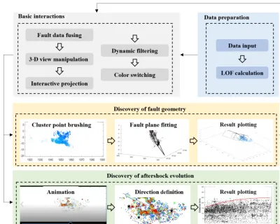
Figure 1.Flowchart of the proposed approach.
2.1 Visual design
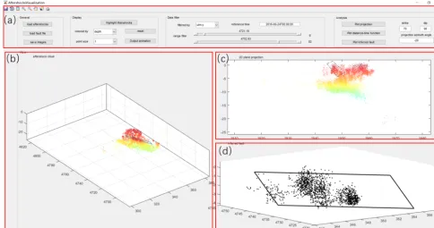
As shown in Fig. 2, the user interface includes four main components. The first component is the operation tools panel with all the buttons, sliders, text boxes, and labels. It in-cludes most interactions in the visual analytics. The second component is the 3-D view panel for presenting cloud points and fault planes. The third component is the 2-D view panel for presenting the points in the 2-D projection plane. The fourth component is a temporal panel that switches between 3-D fault plane fitting plotting and propagation distance–time plotting, corresponding to the explorations of the fault geom-etry and aftershock dynamics, respectively.
2.2 Interactive operations
The easy-to-use interactions represent a significant differ-ence between the proposed method and conventional after-shock interpretation methods. The traditional static displays prevent the analyst from directly and rapidly exploring the af-tershock data. However, the easy-to-use interactive displays can lead to deeper insights into 3-D aftershock cloud point data and the discovery of new fault structures or
spatiotem-poral evolution patterns. These interactive operations are de-scribed as follows.
Three-dimensional view manipulation. The point cloud data can be displayed in a 3-D view control (Fig. 2b). Some typical 3-D interactions are available including zooming, panning, rotating, data tips, and data brushing (Fig. 2a), al-lowing interactive exploration and editing of the plotted data to improve the visual display.
Interactive projection.The cross-section plot is the main visualization approach for exploring the complex fault ge-ometry (Fig. 2c). The faults are normally represented by lin-ear features when the aftershocks are projected onto a plane perpendicular to the fault. We offer an interface to input the strike and dip of the projection plane for rapid plotting of a desired plane projection profile.
Figure 2.Visual interface of our approach consisting of four interrelated components:(a)operation tools,(b)a 3-D view,(c)a 2-D projection view, and(d)a temporal view for plotting a fitted fault plane or distance–time function.
Color switching. The feature for coloring the aftershock points can be quickly switched between the depth, LOF, time, and magnitude, allowing the users to effectively understand the data from different dimensions (Fig. 2a).
Fault plane fitting.To test the probability of an identified fault, the users first brush the points that form a linear feature in the cross-section plot (Fig. 2c). A fault plane will be au-tomatically fitted to these points based on a robust estimator (Fig. 2d). This interaction combines expert knowledge and visual computing, allowing the user to quantitatively locate the potential fault structure.
Fault data fusing.Users can import the faults to the 3-D view in order to assist in the visualization and analysis of the aftershock point cloud (Fig. 2b). These faults can be hypo-thetical seismogenic faults or background fault systems.
Animation. The aftershocks can be plotted gradually to form an animation in both the 3-D view and the 2-D cross-section plot (Fig. 2b and c). An animated visualization has unique advantages and aids the viewers in interpreting the evolution of the aftershocks, making comparisons between different points in time, chunking the aftershock points into smaller datasets, focusing attention, and anticipating and un-derstanding the spatiotemporal changes in the aftershocks.
Propagation distance–time plotting. To further quantify the migration process of the aftershocks, users can define a propagation direction (Fig. 2c) and plot the distance along this direction as a function of time (Fig. 2d). The temporal
trend may reveal the mechanism (e.g., fluid diffusion) under-lying the aftershock migration.
2.3 LOF calculation
Because of the limitations due to the resolution of seismic data inversion, there is some uncertainty in the location of the aftershocks, so that some earthquake points show large devi-ations from the fault plane. Usually, the original aftershock data do not contain any information about this uncertainty, and we cannot eliminate these outliers. In this study, we pro-posed to use the LOF, which is commonly used in the iden-tification of the outliers in the lidar point cloud (Wang et al., 2019) to detect the anomalous points that deviate distinctly from the fault plane. The LOF (Breunig et al., 2000) is based on the concept of local density, which is estimated by the reachability distance of the object to itsknearest neighbors. Points with a substantially lower density than their neighbors are considered outliers. By comparing the local reachability density of the object to those of its neighbors, its LOF value can be obtained. The LOF is calculated as follows.
Letkd(p)be the k distance of a point p, defined as the distance from point p to thekth nearest neighbor. The reach-ability distance between points p and o is then given by
Figure 3.An example of LOF scores for 2-D points. Each point is colored by its LOF score. The radius of red circles on five selected points is in direct proportion to their LOF score (plotted in the cen-ter). It is observed that the central points with high density have low LOF scores, while the surrounding points have high ones.
The local reachability density of an object p is then defined by
lrdk(p)=
|Nk(p)|
P
o∈Nk(p)rdk(p,o)
, (2)
whereNk(p)is thekth nearest neighborhood, defined as the set of points within the distance of thekdistance (p).
The LOF for point p is then obtained by
LOFk(p)=
P
o∈Nk(p)lrdk(o)
|Nk(p)|lrdk(p) . (3)
Figure 3 shows an example of the calculated LOF values, where an LOF value significantly larger than 1 indicates a sparse region.
2.4 Two-dimensional projection
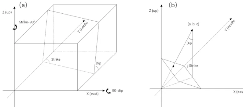
Projecting the 3-D aftershock point cloud to a 2-D plane can significantly enhance the fault geometry features. As men-tioned above, we offer an interactive way to rapidly compute the projection when a plane and projection direction are as-signed. To make the interactive operation user-friendly for geologists, we use geological terms, i.e., strike and dip (to define the orientation of the projection plane), and azimuth angle (to define the projection angle). We firstly calculate 3-D geographic coordinates of the projected points on the pro-jection plane for aftershocks according to the line–plane in-tersection equation. The 3-D geographic coordinates are then transformed to a 2-D local coordinate system by two element rotations: azaxis rotation by an angle of strike−90◦and an
x axis rotation by an angle of−dip, as shown in Fig. 4a.
The rotation matrices (RzandRx) are given by
Rz strike−90◦=
" cos(strike−90◦) −sin(strike−90◦) 0
sin(strike−90◦) cos(strike−90◦) 0
0 0 1
#
(4) and
Rx(90−dip)=
1 0 0
0 cos(−dip) −sin(−dip)
0 sin(−dip) cos(−dip)
. (5)
The projected coordinates (P) from the aftershock point (u)
is given by
P=RxRzu, (6)
where thexandycoordinates ofPcorrespond to the coordi-nates in the projection plane, and thezcoordinate represents the distance to the plane.
2.5 Plane fitting
When the analyst identifies a potential linear feature from the cross-section plot, the plane fitting can rapidly evaluate the possible feature and provides the precise geometric param-eters. In this study, we used an algorithm based on the sin-gular value decomposition (SVD) to fit a plane to the given 3-D aftershock points. The calculation of the parameters of the plane (ax+by+cz=d) based on the singular value de-composition method is carried out as follows.
Given a set of points(xi, yi, zi, i=1. . .n)and their center point (x,¯ y,¯ z¯), we form a matrixAas given by
A=
x1− ¯x y1− ¯y z1− ¯z
x2− ¯x y2− ¯y z2− ¯z
x3− ¯x y3− ¯y z3− ¯z
. . .
. . .
xn− ¯x yn− ¯y zn− ¯z
. (7)
We apply an SVD to matrixA:
A=U DVT. (8)
The parameter vector [a, b, c] is just the smallest singular vector corresponding to the least singular value, and the last parameterdcan be obtained by
d=ax¯+by¯+cz.¯ (9)
To avoid disturbance from noisy points, we include an iter-ative step to identify outliers and exclude them from plane fitting. This step is carried out using the following algorithm:
1. Fit a plane using the available points.
2. Calculate the distance (D) of the points to the plane. 3. Calculate the root mean square error (RMSE) of all of
Figure 4. (a)Illumination of a projection to a plane defined by strike and dip.(b)Strike and dip parameter calculation from a normal vector of a fitted plane.
4. Find points with distances 3 times larger than RMSE and define them as outliers.
5. Remove these points, and then return to step 1.
6. Stop when there is no outlier found, and return the plane parameter.
Given the normal vector of the fitted plane (a, b, c), the strike and dip of the fault plane are given by (Fig. 4b)
strike=atan2(sign(c)×a,sign(c)×b) (10) and
dip=acos(c/pa2+b2+c2), (11) where atan2(Y, X)is the four quadrant arctangent of the el-ements XandY,−π <=atan2(Y, X) <=π, and sign(.) is the signum function that returns 1 for a positive element and
−1 for a negative element. 2.6 Prototype system
The proposed visualization approach has been implemented in a software package (Aftershock Visualization, AFV1.0; https://github.com/caigenszu, last access: 22 August 2019) and is freely accessible to the scientific community. This pro-totype system was developed in MATLAB with a graphical user interface (GUI), providing point-and-click control for all operations. An analyst with no programming background does not need to learn a new language or type commands to run the application. Meanwhile, the source code of the pack-age is also provided so that advanced users can easily read the data and results throughout the visualization processing, and they can modify the package to include their custom-built modules. This package requires an input file consisting of the aftershock point cloud table in plain text with each row
representing a point and the columns representing UTM-x, UTM-y, depth, magnitude, time (days from reference time), LOF, and an event flag (whether or not the shock is the main shock) in that order. An alternative input file is the fault plane used to assist data interpretation. Each fault plane is repre-sented by one row, and the columns represent strike, dip, cen-ter UTM-x, center UTM-y, length, upper depth, and bottom depth.
3 Case study: the 2016 Central Italy earthquake sequence
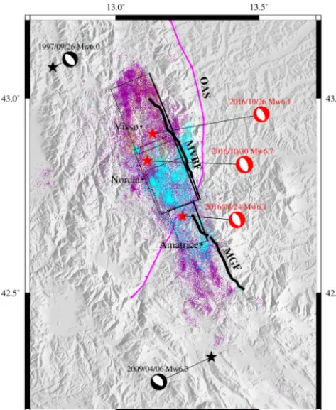
On 24 August 2016 (01:36 UTC, local time 03:36), a de-structive earthquake (Mw 6.2) occurred in Central Italy (the Amatrice earthquake). The epicenter was located at 42.70◦N, 13.23◦E, between the towns of Norcia and Am-atrice. Two months later, two major earthquakes were trig-gered to the northwest of the Amatrice earthquake on 26 Oc-tober (19:18 UTC) and 30 OcOc-tober (06:40 UTC) (Papadopou-los et al., 2017), with individual moment magnitudes of 6.1 (Visso earthquake) and 6.6 (Norcia earthquake). The earthquake sequence occurred across several fault systems (Fig. 5), including the Mt. Vettore–Mt. Bove Fault system (VBFS) and the Mt. Gorzano Fault system (GFS). The VBFS is a SW-dipping fault system composed of different splays and segments. The fault system scarps are exposed along the SW foothills of Mt. Vettore, Mt. Porche, and Mt. Bove, with a length of∼27 km. The GFS is a SW-dipping fault with a
Figure 5.Seismotectonic setting of the Central Italy earthquake se-quence. The three major earthquakes in the sequence are denoted by the red stars and beach ball symbols, and the two recent large histor-ical events are colored in black. The dashed black rectangles repre-sent the surface projection of the fault planes adopted in this study. The bold black lines are the two seismogenic normal fault systems, namely, the Mt. Vettore–Mt. Bove Fault system (VBFS) and the Mt. Gorzano Fault system (GFS). The pink line shows the simplified trace of the preexisting compressional front named the Olevano– Antrodoco–Sibillini (OAS) Thrust. Aftershocks are marked by the small dots with different colors. The blue, purple, and yellow points represent the events taking place on 24 August–24 October 2016, 24–30 October 2016, and 30 October 2016–8 October 2017, respec-tively.
the seismicity to the first 8 km of the crust (Chiaraluce et al., 2017).
Many recent studies reported in the literature have re-vealed a very complex fault geometry for this earthquake sequence. In addition to the main range-front normal fault-ing structures that were adopted in many early studies (Liu et al., 2017; Tinti et al., 2016), recent studies find increasing evidence for some additional minor antithetic and synthetic faults (Chiaraluce et al., 2017; Scognamiglio et al., 2018; Walters et al., 2018; Cheloni et al., 2017). The activation of this secondary fault structure has important implications for evaluating the seismic hazard in this section of the Cen-tral Apennines. The complex fault geometry also plays an important role in channeling fluid diffusion and affects the spatial order of the cascading earthquakes. The aftershock
distribution provides direct evidence for the fault geome-try and underground dynamics. By interactively visualizing these data, we can obtain useful information regarding both the fault geometry and earthquake dynamics. Additionally, a relocated aftershock dataset has been provided in the work of Chiaraluce et al. (2017), making this earthquake sequence an ideal case for applying our proposed interactive visualization method. Below, we demonstrate the benefits of our method in identifying fault geometry and aftershock migration. 3.1 Fault geometry identification
According to previous studies, several fault segments are in-volved in this earthquake sequence. Some of these are the main fault segments located in the GFS–VBFS, while others are secondary fault segments including a NE-dipping nor-mal fault antithetic to the GFS–VBFS and a preexisting com-pressional structure that is likely related to a segment of the Olevano–Antrodoco–Sibillini Thrust. We will show how our interactive visualization method can facilitate the recognition of these structures.
Following the flowchart shown in Fig. 1, we first import the relocated aftershock data from the results obtained by Chiaraluce et al. (2017) to the 3-D view. Some of the basic in-teractions provided by this package, i.e., zooming, panning, rotating, data tips, and data brushing, can be used to explore the data. LOF values were then calculated for all points to identify the aftershock outliers. We can interactively select to show some of the points according to their location, depth, magnitude, LOF, and time, and we can project them to a de-sired plane. After we find a linear feature in the projection plane, we select the points comprising the linear feature and automatically fit a plane to the feature (Fig. 6).
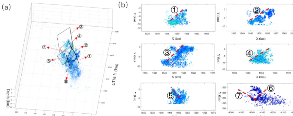
First, we identify the four main fault planes by projecting the cloud point to a plane with a 70◦strike and a 90◦dip. This plane is approximately perpendicular to the GFS–VBFS, and it should reveal the cross sections of the fault plane well. To better illuminate the linear features of the faults, we filter the aftershock points according to the fault location and the span-ning time of the aftershocks on the fault. To denoise the point cloud, the aftershocks with the LOF value larger than 2 are filtered. We then select the points around the linear feature for each fault plane, and we automatically obtain the suggested geometry parameters of the fitted plane as shown in Table 1, finding that the obtained parameters are in overall agreement with the main seismogenic fault planes in previous studies.
Figure 6.Fault geometry identification and plane fitting.(a)A three-dimensional view of seven identified fault segments and an aftershock point cloud. Thick lines represent the surface traces of the faults, and the dashed lines are the underground fault boundaries.(b)Projections of the 3-D aftershocks. Red dashed lines denote the seven fitted fault planes.
Table 1.Geometry parameters of the inferred fault from the aftershock point cloud. Strike and dip are given in degrees; all other parameters are measured in kilometers.
Strike Dip UTM-X UTM-Y Length Upper depth Bottom depth
159.06 55.64 357.36 4738.96 18.57 0.00 7.26
140.40 32.08 351.23 4752.59 15.76 0.00 9.31
166.93 35.92 346.80 4775.10 30.88 0.00 10.00
153.88 37.28 351.05 4753.25 29.86 0.00 7.09
−19.12 60.71 348.21 4734.50 18.87 0.00 4.55
−113.54 46.51 351.73 4734.97 8.45 0.00 11.17
7.81 85.33 348.16 4745.97 32.31 0.00 11.52
Fig. 6. Fault fitting gives a strike of−38◦and a dip of 59.8◦ for the Norcia antithetic fault. However, other fault structures revealed in the literature are not very obvious in the after-shock cloud point. We then project the point cloud to a sim-plified seismogenic fault (strike=160◦, dip=50◦) along a
horizontal vector with an azimuth of 15◦, using the projection
settings from Walters et al. (2018). We filter the points by the magnitude, location, timing, and LOF, and then, two linear structures are observed as shown in Fig. 6. The structure on the right is the NW-dipping Pian Piccole fault that generates a significant surface displacement signal in the interferometric synthetic aperture radar (InSAR) measurements. The struc-ture on the left is an east-dipping fault that was only inferred in Walters et al. (2018). We pick the points around these lin-ear structures for plane fitting and obtain a strike of−114◦ and a dip of 46.5◦ for the Pian Piccole fault and a strike of 7.8◦and a dip of 85.3◦for the inferred fault.
3.2 Migration of aftershocks
Besides the static analysis of aftershocks to find the fault ge-ometry, the timing information of aftershocks has the poten-tial to reveal earthquake dynamics related to fluid diffusion, afterslip, and/or pressure transients. Fluid diffusion is a main factor in triggering seismicity as observed in many tectonic regimes (Vidale and Shearer, 2006). It was also proposed to have been present in the nearby 2009 L’Aquila earthquake (Malagnini et al., 2012). The migration of the aftershocks could provide some evidence for such diffusive processes. Walters et al. (2018) found a significant fluid-driven after-shock migration between the Amatrice earthquake and Visso earthquake controlled by the fault intersection in this earth-quake sequence.
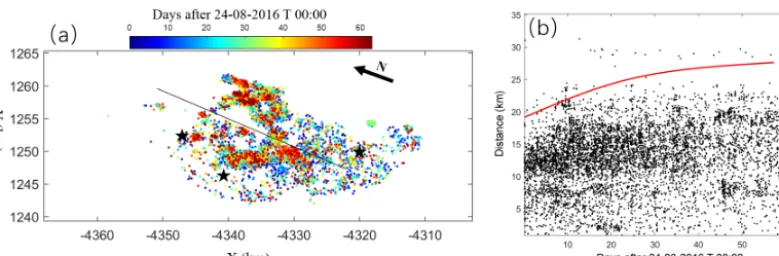
Figure 7. Observation of aftershock migration.(a)Aftershock on the projection plane colored by time. The arrow represents north. It is observed that most aftershock points in the north happened more recently than in the south, implying a northward migration trend. (b)Propagation distance as a function of time. The red line represents the temporal trend that the propagation distances increase with time.
the northward direction, implying the clear directionality of the aftershock migration. We then use the animation opera-tion to plot the aftershock points step by step as a funcopera-tion of time in both the 2-D projection plane and the 3-D view. The directional propagation of the aftershocks can be observed much more clearly.
Next, we can define a starting point and an assumed direc-tion in the projecdirec-tion plane. After drawing the starting point and the propagation line, the distances of the aftershocks to the starting point along this direction can be calculated au-tomatically. They are then plotted as a function of time to further reveal the time evolution of the aftershocks. Follow-ing the work of Walters et al. (2018), we defined a startFollow-ing point in the peak slip of the Amatrice earthquake and a di-rection perpendicular to the Pian Piccolo fault. A clear tem-poral trend of the aftershocks was then observed in the plot (Fig. 7b). Therefore, the observed spatiotemporal pattern of aftershock migration can be interpreted by the seismologist to understand the earthquake mechanism and infer the possi-ble controlling factor for the fault rupture. In this case, the diffusive-like aftershock temporal trend can be further terpreted using a pore fluid source model. Through the in-teractive visualization operations, we can observe that after-shock propagation is consistent with a diffusive process and can also observe the spatial concentration of the aftershocks along the fault intersection. This information can be used to derive the conclusion, as described in the work of Walters et al. (2018), that the intersecting structures act to channel the fluids and control the timing and order of the subsequent earthquakes.
4 Conclusion
We present a novel interactive approach and develop a proto-type system to illustrate 3-D aftershock point clouds that can help the geophysicist and seismologist to better understand the geometry of a complex fault system and the spatiotempo-ral pattern of the aftershocks. Moreover, it can be applied in
an educational scenario to facilitate student learning. In this approach, we design a set of interactive operations to facil-itate the exploration of the data. Fast computation of LOF, 2-D projection, and plane fitting are implemented in addition to the visualization to reveal additional, hidden information, which is not obvious in the original data. Additionally, the point cloud can be visualized in many ways (e.g., 3-D view, 2-D plane projection, and animation), aiding viewers in in-terpreting the aftershock point cloud. A wide range of data filtering options (e.g., by magnitude, depth, location, time, and LOF) enable the users to avoid interference from invalid data in order to focus on the useful information.
It is widely accepted that visual analytics with interactive visual interfaces can amplify human cognitive capabilities, and it is suitable for solving some complex problems rely-ing on closely coupled human and machine analysis. When applied to the aftershock catalog, visual analytics can there-fore help to discover some new fault planes or weak signals of aftershock migrations, which might be hard to observe di-rectly from the data. Specifically, the designed visual analyt-ics procedure can assist the knowledge discovery from the aftershock catalog in several ways:
1. by accelerating the fault segment discovery processing through 3-D view manipulation (e.g., zooming, pan-ning, and rotating);
2. by enhancing the recognition of fault segment patterns through rapid visual computing functions (e.g., interac-tive projection, plane fitting, and fault data fusing); 3. by reducing the influence from low-quality or
irrele-vant aftershock points through various filtering methods (e.g., depth, LOF, time, and magnitude filtering); 4. by enabling the aftershock migration exploration by
providing more cognitive resources (e.g., animation and propagation distance–time plotting).
complex visualization operations in a user-friendly interac-tive manner. We can conveniently infer the fault geometry for both the main faults and the secondary faults, and we clearly observe the spatiotemporal pattern of the fluid-driven after-shock migration. In future work, we would like to examine the capability of this tool for more aftershock point data ap-plications, such as analyzing tremor migration and tracking aseismic slip. Also, we plan to include more kinds of fault in-formation (e.g., InSAR, GPS, source model, and fault scarp) in the visualization in order to further facilitate the analysis of earthquake fault behavior.
Data availability. The research data are included in the Supple-ment.
Supplement. The supplement related to this article is available on-line at: https://doi.org/10.5194/se-10-1397-2019-supplement.
Author contributions. This work was conducted by CW and JJ un-der the supervision of QL. The paper was prepared by CW and JJ with contributions from all co-authors.
Competing interests. The authors declare that they have no conflict of interest.
Financial support. This research has been supported by the Shen-zhen Scientific Research and Development Funding Program (grant nos. KQJSCX20180328093453763, JCYJ20180305125101282, JCYJ20170817104236221, and JCYJ20170412142144518), the Open Fund of the State Key Laboratory of Earthquake Dynam-ics (grant no. LED2016B03), the NSFC (grant nos. 61802265 and 41974006), Guangdong Provincial Natural Science Foundation (grant no. 2018A030310426), and the Open Fund of Key Labora-tory of Urban Land Resources Monitoring and Simulation, Ministry of Land and Resource (grant no. KF-2018-03-004).
Review statement. This paper was edited by Caroline Beghein and reviewed by two anonymous referees.
References
Barbot, S., Lapusta, N., and Avouac, J. P.: Under the hood of the earthquake machine: toward predictive modeling of the seismic cycle, Science, 336, 707–710, 2012.
Breunig, M. M., Kriegel, H., Ng, R. T., and Sander, J.: LOF: iden-tifying density-based local outliers, International Conference on Management of Data, 29, 93–104, 2000.
Cheloni, D., De Novellis, V., Albano, M., Antonioli, A., Anzidei, M., Atzori, S., Avallone, A., Bignami, C., Bonano, M., and Cal-caterra, S.: Geodetic model of the 2016 Central Italy earthquake
sequence inferred from InSAR and GPS data, Geophys. Res. Lett., 44, 6778–6787, 2017.
Chiaraluce, L., Di Stefano, R., Tinti, E., Scognamiglio, L., Michele, M., Casarotti, E., Cattaneo, M., De Gori, P., Chiarabba, C., and Monachesi, G.: The 2016 Central Italy seismic sequence: a first look at the mainshocks, aftershocks, and source models, Seismol. Res. Lett., 88, 757–771, 2017.
Elliott, J., Copley, A., Holley, R., Scharer, K., and Parsons, B.: The 2011Mw7.1 van (eastern Turkey) earthquake, J. Geophys. Res.-Sol. Ea., 118, 1619–1637, 2013.
Elliott, J. R., Parsons, B., Jackson, J. A., Shan, X., Sloan, R. A., and Walker, R. T.: Depth segmentation of the seismogenic conti-nental crust: The 2008 and 2009 Qaidam earthquakes, Geophys. Res. Lett., 38, L06305, https://doi.org/10.1029/2011GL046897, 2011.
Hengesh, J. V. and Whitney, B. B.: Transcurrent reactivation of Australia’s western passive margin: An example of intraplate de-formation from the central Indo-Australian plate, Tectonics, 35, 1066–1089, 2016.
Irmak, T. S., Do˘gan, B., and Karaka¸s, A.: Source mechanism of the 23 October, 2011, Van (Turkey) earthquake (Mw=7.1) and aftershocks with its tectonic implications, Earth Planets Space, 64, 991–1003, 2012.
Li, Y., Jia, D., Shaw, J. H., Hubbard, J., Lin, A., and Wang, M.: Strutural interpretation of the co-seismic faults of the Wenchuan earthquake: 3D modeling of the Longmen Shan fold-and-thrust belt, J. Geophys. Res., 390, 275–286, https://doi.org/10.1029/2009JB006824, 2010.
Liu, C., Zheng, Y., Xie, Z., and Xiong, X.: Rupture features of the 2016Mw 6.2 Norcia earthquake and its possible relation-ship with strong seismic hazards, Geophys. Res. Lett., 44, 1320– 1328, 2017.
Liu, R., Chen, S., Ji, G., Zhao, B., Li, Q., and Su, M.: Interactive stratigraphic structure visualization for seismic data, J. Visual Lang. Comput., 48, 81–90, 2018.
Malagnini, L., Lucente, F. P., Gori, P. D., Akinci, A., and Munafo, I.: Control of pore fluid pressure diffusion on fault failure mode: Insights from the 2009 L’Aquila seis-mic sequence, J. Geophys. Res.-Sol. Ea., 117, B05302, https://doi.org/10.1029/2011JB008911, 2012.
Manighetti, I., Caulet, C., Barros, L., Perrin, C., Cappa, F., and Gaudemer, Y.: Generic along-strike segmentation of Afar nor-mal faults, East Africa: Implications on fault growth and stress heterogeneity on seismogenic fault planes, Geochem. Geophys. Geosyst., 16, 443–467, 2015.
McCormick, B. H.: Visualization in scientific computing, ACM SIGBIO Newsletter, 10, 15–21, 1988.
Papadopoulos, G., Ganas, A., Agalos, A., Papageorgiou, A., Tri-antafyllou, I., Kontoes, C., Papoutsis, I., and Diakogianni, G.: Earthquake triggering inferred from rupture histories, DInSAR ground deformation and stress-transfer modelling: the case of Central Italy during August 2016–January 2017, J. Pure Appl. Geophys., 174, 3689–3711, 2017.
Raposo, A., Reis, L., Rodrigues, V., Pinheiro, R., Elias, P., and Cherullo, R.: A system for integrated visualization in oil explo-ration and production, IEEE Comput. Graph., 36, 10–16, 2016. Scognamiglio, L., Tinti, E., Casarotti, E., Pucci, S., Villani, F.,
Cocco, M., Magnoni, F., Michelini, A., and Dreger, D.: Com-plex fault geometry and rupture dynamics of theMw6.5, 2016, October 30th central Italy earthquake, J. Geophys. Res.-Sol. Ea., 123, 2943–2964, 2018.
Tinti, E., Scognamiglio, L., Michelini, A., and Cocco, M.: Slip het-erogeneity and directivity of the ML 6.0, 2016, Amatrice earth-quake estimated with rapid finite-fault inversion, Geophys. Res. Lett., 43, 10745–10752, 2016.
Vidale, J. E. and Shearer, P. M.: A survey of 71 earthquake bursts across southern California: Exploring the role of pore fluid pres-sure fluctuations and aseismic slip as drivers, J. Geophys. Res.-Sol. Ea., 111, B05312, https://doi.org/10.1029/2005JB004034, 2006.
Walters, R. J., Gregory, L. C., Wedmore, L. N. J., Craig, T. J., McCaffrey, K., Wilkinson, M., Chen, J., Li, Z., Elliott, J. R., Goodall, H., Iezzi, F., Livio, F., Michetti, A. M., Roberts, G., and Vittori, E.: Dual control of fault intersections on stop-start rupture in the 2016 Central Italy seismic sequence, Earth Planet. Sc. Lett., 500, 1–14, https://doi.org/10.1016/j.epsl.2018.07.043, 2018.
Wang, C., Shu, Q., Wang, X., Guo, B., Liu, P., and Li, Q.: A random forest classifier based on pixel comparison features for urban Li-DAR data, ISPRS Journal of Photogrammetry Remote Sensing, 148, 75–86, 2019.
Ward, M. O., Grinstein, G., and Keim, D.: Interactive data visualiza-tion: foundations, techniques, and applications, AK Peters/CRC Press, New York, 2015.
Wong, P. C. and Thomas, J.: Visual analytics, IEEE Comput. Graph., 24, 20–21, 2004.