Nonlin. Processes Geophys., 20, 803–818, 2013 www.nonlin-processes-geophys.net/20/803/2013/ doi:10.5194/npg-20-803-2013
© Author(s) 2013. CC Attribution 3.0 License.
Nonlinear Processes
in Geophysics
Open Access
Joint state and parameter estimation with an iterative ensemble
Kalman smoother
M. Bocquet1,2and P. Sakov3
1Université Paris-Est, CEREA joint laboratory École des Ponts ParisTech and EDF R&D, France 2INRIA, Paris Rocquencourt research centre, France
3Bureau of Meteorology, Melbourne, Australia
Correspondence to: M. Bocquet ([email protected])
Received: 4 June 2013 – Revised: 2 September 2013 – Accepted: 4 September 2013 – Published: 23 October 2013
Abstract. Both ensemble filtering and variational data assim-ilation methods have proven useful in the joint estimation of state variables and parameters of geophysical models. Yet, their respective benefits and drawbacks in this task are dis-tinct. An ensemble variational method, known as the itera-tive ensemble Kalman smoother (IEnKS) has recently been introduced. It is based on an adjoint model-free variational, but flow-dependent, scheme. As such, the IEnKS is a can-didate tool for joint state and parameter estimation that may inherit the benefits from both the ensemble filtering and vari-ational approaches.
In this study, an augmented state IEnKS is tested on its estimation of the forcing parameter of the Lorenz-95 model. Since joint state and parameter estimation is especially use-ful in applications where the forcings are uncertain but never-theless determining, typically in atmospheric chemistry, the augmented state IEnKS is tested on a new low-order model that takes its meteorological part from the Lorenz-95 model, and its chemical part from the advection diffusion of a tracer. In these experiments, the IEnKS is compared to the ensemble Kalman filter, the ensemble Kalman smoother, and a 4D-Var, which are considered the methods of choice to solve these joint estimation problems. In this low-order model context, the IEnKS is shown to significantly outperform the other methods regardless of the length of the data assimilation win-dow, and for present time analysis as well as retrospective analysis. Besides which, the performance of the IEnKS is even more striking on parameter estimation; getting close to the same performance with 4D-Var is likely to require both a long data assimilation window and a complex modeling of the background statistics.
1 Introduction
Data assimilation in geophysics is often concerned with the estimation of the state of the system (e.g. atmosphere, ocean). Yet, non-observed parameters of the model can also be seen as control variables. They can indirectly be estimated through the assimilation of observations. In such context, data assim-ilation can be a powerful inverse modeling tool.
With the progress in techniques as well as the rise in pop-ularity of data assimilation in geosciences, this topic has be-come of increasing interest. Parameter estimation is useful because it can account for model error through a parametric representation of the uncertain processes, and could serve as a tool to enhance the system state estimation. For instance, it is now accepted that air quality forecasting can benefit con-siderably from the online estimation of forcing parameters. Parameter estimation is also a fundamental tool per se in the estimation of the parameters which are often of physical or societal interests. For instance, again regarding air quality, data assimilation can help assess effective kinetic rates of in-terest to chemists, or it can help assess regulated pollutant emissions of interest to policy makers.
1.1 Data assimilation techniques for parameter estimation
As is the case with data assimilation for state estimation, two types of approach have been used for parameter estimation: filtering methods and variational methods.
The estimation of parameters by the filtering approaches is based on the augmentation of the state vector with the pa-rameter variables. If the state space has dimensionMand if the number of parameters isP, then the augmented control
804 M. Bocquet and P. Sakov: State and parameter estimation with the IEnKS
vector has dimension M+P. Through the assimilation of observations, the joint analysis of the state variables and the parameters aims at building covariances (or higher-order de-pendencies for non-Gaussian filters) between them; these are crucially needed because of the non-observability of most pa-rameters. The augmented state principle is likely to be used with any type of filter: extended Kalman filters (e.g., Kon-drashov et al., 2008), ensemble Kalman filters (e.g., Aksoy et al., 2006; Wirth and Verron, 2008; Barbu et al., 2009), par-ticle filters (e.g., Vossepoel and van Leeuwen, 2007; Weir et al., 2013), and stochastic sampling and genetic algorithms (e.g., Jackson et al., 2004; Liu et al., 2005; Bocquet, 2012; Posselt and Bishop, 2012). In an enlightening review, Ruiz et al. (2013) have discussed the use of ensemble Kalman fil-ters (EnKFs) for parameter estimation. When the filtering method accounts for asynchronous observations by build-ing covariances between parameter errors defined at dis-tinct times, the method is usually referred to as a smoother (Evensen, 2003; Hunt et al., 2004; Sakov et al., 2010; Cosme et al., 2010).
The estimation of parameters with the variational ap-proach is based on the explicit dependence of the cost func-tion in not only the state variables, but also the parameters. If the dependence is not explicit, one should at least be able to compute the gradient of the cost function with respect to the parameters. The four-dimensional variational method, or 4D-Var (Le Dimet and Talagrand, 1986; Talagrand and Courtier, 1987; Rabier et al., 2000), has the distinct advantage of be-ing a natural smoother since it works within a temporal win-dow to assimilate asynchronous observations. However, it requires the use of the adjoint evolution model to compute gradients of the cost function. Computing the gradient with respect to the model parameters requires the same adjoint model, and also the extra effort of computing the explicit derivative of the cost function with respect to the parameters, in terms of the adjoint variables. It has been used for param-eter estimation by, e.g., Pulido and Thuburn (2006), Bocquet (2012), and Kazantsev (2012).
This list of contributions to the field is far from being ex-haustive and merely illustrates some of the methodologies used in atmospheric, ocean and climate sciences. In partic-ular, there is a vast literature in atmospheric chemistry ded-icated to the inversion of sources of pollutants and tracers. The extended and ensemble Kalman filters and variational methods (3D-Var and 4D-Var) have been employed in this field for over two decades (Zhang et al., 2012, and refer-ences within). Owing to the (quasi-)linearity of some chem-ical species, simpler four-dimensional smoothing analysis merely using a Best Linear Unbiased Estimator (BLUE) have also been extensively used to estimate sources.
1.2 The iterative ensemble Kalman smoother
The iterative ensemble Kalman smoother (IEnKS) has been recently proposed (Bocquet and Sakov, 2013) as an extension
of the iterative ensemble Kalman filter (Sakov et al., 2012; Bocquet and Sakov, 2012). It is meant to solve the variational problem of 4D-Var with the help of a 4D ensemble. As such, it is a 4D ensemble variational method of the type used in the work by Buehner et al. (2010), Chen and Oliver (2012) and Fairbairn et al. (2013), and has (more remote) connections with ensemble of variational methods (Raynaud et al., 2009; Bowler et al., 2013). It does not require the use of the adjoint observation and evolution models since the sensitivities are estimated with the ensemble (Gu and Oliver, 2007; Liu et al., 2008). Moreover, the IEnKS generates the posterior ensem-ble using Gaussian assumptions and forecasts the ensemensem-ble to the next update step in the same way an ensemble square root Kalman filter does. Note that the scheme is not a hybrid method since it does not combine two distinct methods.
Because the IEnKS fundamentally solves a variational problem, it may require iterations for the cost function min-imization. The number of iterations depends on the nonlin-earity of the system. This number is expected to be small (1 or 2) for weak nonlinearity (typical of synoptic scale meteo-rology).
Using perfect model assumptions, Bocquet and Sakov (2013) have tested the IEnKS on two low-order models in different regimes representing different nonlinearities and lengths of the data assimilation window (DAW). The IEnKS (often significantly) outperforms EnKF and the standard en-semble Kalman smoother (EnKS) in all these regimes, not only regarding the smoothing performance (retrospective state estimation) but also regarding the filtering performance (state estimation at present and future time). Here, we will also show that the IEnKS also outperforms 4D-Var in this context.
In addition, the IEnKS has been shown on these models to be able to handle long DAWs, especially when assimilat-ing observations several times (in a mathematically consis-tent manner).
Because the IEnKS offers the advantages of both filtering and variational methods, and because it is capable of operat-ing on long DAWs, it has considerable potential as an effi-cient parameter estimation method.
1.3 Objective and outline
The objective of this article is to introduce a straightforward extension of the IEnKS to joint state and parameter estima-tion, and to test the potential of the approach on low-order models. The physical context is that of chaotic geophysical models, and of atmospheric chemical/tracer models, in which a joint state and parameter estimation is, in our opinion, a key to successful forecasts.
M. Bocquet and P. Sakov: State and parameter estimation with the IEnKS 805
tests will be performed: a comparison with the state-of-the-art EnKF and standard EnKS, as well as with a 4D-Var, and with a new cycling of the IEnKS DAWs. Then the IEnKS will be tested for joint state and parameter estimation on the Lorenz-95 model (Lorenz and Emmanuel, 1998). In Sect. 4, an original extension of the Lorenz-95 with the advection of a tracer will be introduced. It is meant to represent the dy-namics of an online atmospheric chemistry model, or mete-orological models with a constituent such as moisture, with two unobserved parameters: the Lorenz-95 forcing parame-ter, and the emission flux. The IEnKS, the EnKF/EnKS, and a 4D-Var will be tested and compared in this context. The re-sults will be discussed in Sect. 5. Conclusions will be drawn in Sect. 6.
2 The iterative ensemble Kalman smoother for joint state and parameter estimation
2.1 The algorithm
A Bayesian derivation of the IEnKS can be found in Bocquet and Sakov (2013). However, we would like to introduce the IEnKS comprehensively in this article: reference to Bocquet and Sakov (2013) will only be made regarding details that are not directly relevant to this study. Here, we describe the algorithm with its main justifications, and then provide its pseudo-code.
2.1.1 The core algorithm
Observation vectorsy∈Rdare assumed to be collected ev-ery time step1t. Time is discretized into the timestk when
the observations are collected. The numberd of scalar ob-servations withinycan be time-dependent. The observations are related to the state vector through a possibly nonlinear, possibly time-dependent observation operator Hk. The
ob-servation errors are assumed to be Gaussian-distributed, un-biased, and uncorrelated in time, and to have an observation error covariance matrix Rk.
The analysis step of the assimilation scheme is performed over a window of lengthL1tin time units. Unless otherwise stated, time indexkis relative to present time. With this con-vention, present time is set to be alwaystL, so that the initial
condition of the DAW is conveniently alwayst0.
Let us first describe the update step. At t0 (i.e. L1t in
the past), the background is obtained from an ensemble of
N state vectors ofRM:x
0,[1], . . . ,x0,[n], . . . ,x0,[N]. Index 0
refers to time while[n]refers to the ensemble member index. They can be stored in a matrix E0= [x0,[1], . . . ,x0,[N]] ∈
RM×N. One can equivalently represent the ensemble with
its meanx0=N1PNn=1x0,[n] and its anomaly matrix A0=
[x0,[1]−x0, . . . ,x0,[N]−x0].
As in the ensemble Kalman filter, this background is ap-proximated as a Gaussian distribution of meanx0, and
co-variance matrix A0AT0/(N−1), the first- and second-order
empirical moments of the ensemble. The background is rarely full rank since the anomalies of the ensemble span a vector space of dimension smaller than or equal to N−1 and in a realistic context NM. Therefore, one solves for the analysis state vectorx0in the ensemble spacex0+
Vec
x[1]−x0, . . . ,x[N]−x0 , which can be written x0= x0+A0w, wherew∈RN is a vector of coefficients in
en-semble space.
The analysis of IEnKS over[t0, tL]is obtained from a cost
function. The restriction of this cost function in state space to the ensemble space yields:
e
J(w)= 1
2(N−1)w
Tw+1
2
L X
k=1
βkδTk(w)R
−1 k δk(w) ,
δk(w)=yk−Hk◦Mk←0
x(00)+A0w
. (1)
The tilde symbol signifies that Jeis a mathematical
ob-ject defined in ensemble space.Mk←0 is the possibly
non-linear transition operator fromt0totk.{βk}1≤k≤Lare scalars
in[0,1]that weight the observations within the DAW. The choice of theβk can be made mathematically consistent and
can have dramatic consequences on the performance of the data assimilation system. We refer to Bocquet and Sakov (2013) for a justification and numerical tests. Nonetheless, the rational for the choice of the{βk}1≤k≤Lwill be discussed
later.
This cost function is iteratively minimized in the ensemble space following the Gauss–Newton algorithm:
w(j+1)=w(j )−He
−1
(j )∇Je(j )(w(j )) , (2)
using the gradient∇Je(j )and an approximate HessianHe(j )
of the cost function: ∇Je(j )= −
L X
k=1
βkYTk,(j )R
−1 k
h
yk−Hk◦Mk←0(x(j )0 ) i
+(N−1)w(j ), (3)
e
H(j )=(N−1)IN+ L X
k=1
βkYTk,(j )R
−1
k Yk,(j ), (4)
x(j )0 =x(00)+A0w(j ). (5) e
H(j )is an approximation of the full Hessian because it
dis-regards the contribution of the second-order derivatives of the innovation vectorsδk(w)in the cost function. The notation
(j )refers to the iteration index of the minimization. At the first iteration one setsw(0)=0. I
N is the identity matrix in
ensemble space. Yk,(j )=[Hk◦Mk←0]0
|x(j )0 A0is the tangent
linear of the operator from ensemble space to the observation space. The estimation of this sensitivity using the ensemble is what allows one to avoid the use of the model adjoint. Two implementations, referred to as the transform and the bundle variants, have been put forward (Sakov et al., 2012; Bocquet and Sakov, 2012). With the bundle scheme, for instance, the
806 M. Bocquet and P. Sakov: State and parameter estimation with the IEnKS
ensemble is rescaled closer to the mean trajectory by a factor
ε. It is then propagated through the model and the observa-tion operators, after which it is rescaled back by the inverse factorε−1. The operation reads:
Yk,(j )≈
1
εHk◦Mk←0
x(j )0 1T+εA0
IN−
11T
N
, (6)
where 1=(1, . . . ,1)T∈RN.
Note that each iterative update Eq. (2) solves the inner quadratic variational problem:
e
J(j )(w)=1
2(N−1)
w−w
(j ) 2
+1 2
L X
k=1 βk
yk−Hk◦Mk←0(x (j ) 0 )
−Yk,(j )(w−w(j )) 2
Rk
, (7)
wherekzk2 G=z
TG−1z.
The iteration is stopped whenkw(j )−w(j−1)k becomes smaller than a predetermined thresholde. Let us denotew?
the solution of the cost function minimization. The symbol
?will be used with any quantity obtained at the minimum. Subsequently, a posterior ensemble can be generated att0:
E?0=x?01T+ √
N−1A0He
−1/2
? U, (8)
where U is an orthogonal matrix that is arbitrary but satisfies U1=1 – meant to keep the posterior ensemble centered on the analysis – andx?0=x0+A0w?.
The Gauss–Newton minimization scheme shown in Eq. (2) can easily be replaced by a quasi-Newton scheme that avoids the computation of the Hessian, or by a Levenberg– Marquardt algorithm that guarantees convergence of the min-imization. These alternatives have been suggested and suc-cessfully tested in Bocquet and Sakov (2012). In the context of the standard models tested in Sects. 3 and 4, the nonlin-earity is mild enough that a Levenberg–Marquardt scheme is unnecessary, and the Gauss-Newton scheme is very efficient. This ends the part of the analysis step that is required to cy-cle the data assimilation scheme. An optional analysis step is required when a state estimation is desired at timest1, . . . , tL,
i.e. up to present time, or when a forecast to future times is desired. This additional step depends on the choice of theβk
and whether the DAWs are overlapping. In the simplest case, when observations are assimilated once and only once, this subsequent analysis takes the form of a forecast of the mean statex?k=Mk←0(x?0), or a forecast of the full ensemble if
one is additionally interested in estimating forecast uncer-tainty E?k=Mk←0(E?0).
During the forecast step of the scheme cycle, not to be confused with the forecast of the analysis step we just men-tioned, the ensemble is propagated forS1t, withSan inte-ger:
E?S=MS←0(E?0) . (9)
4 M. Bocquet, P. Sakov: State and parameter estimation with the IEnKS
and the observation operators, after which it is rescaled back by the inverse factorε−1. The operation reads:
Yk,(j)≈1
εHk◦Mk←0
x(0j)1T+εA0
IN−
11T N
, (6) where1= (1,...,1)T∈RN.
Note that each iterative update Eq. (2) solves the inner quadratic variational problem:
e
J(j)(w) = 1
2(N−1)
w−w(j) 2
+1
2
L
X
k=1 βk
yk−Hk◦Mk←0(x(0j))
−Yk,(j)(w−w(j)) 2
Rk
, (7)
wherekzk2G=zTG−1z.
The iteration is stopped whenkw(j)−w(j−1)kbecomes
smaller than a predetermined thresholde. Let us denotew⋆
the solution of the cost function minimization. The symbol ⋆will be used with any quantity obtained at the minimum. Subsequently, a posterior ensemble can be generated att0: E⋆0=x⋆01T+√N−1A0He−⋆1/2U, (8) where U is an arbitrary orthogonal matrix but satisfying
U1=1meant to keep the posterior ensemble centered on the analysis, andx⋆0=x0+A0w⋆.
The Gauss-Newton minimization scheme Eq. (2) can eas-ily be replaced by a quasi-Newton scheme that avoids the computation of the Hessian, or a Levenberg-Marquardt al-gorithm that guarantees convergence of the minimization. These alternatives have been suggested and successfully tested in Bocquet and Sakov (2012). In the context of the standard models tested in Sections 3 and 4, the nonlinear-ity is mild enough so that a Levenberg-Marquardt scheme is unnecessary, and the Gauss-Newton scheme is very efficient. This ends the part of the analysis step that is required to cy-cle the data assimilation scheme. An optional analysis step is required when a state estimation is desired at timest1,...,tL,
i.e. up to present time, or when a forecast to future times is desired. This additional step depends on the choice of theβk and whether theDAWs are overlapping. In the simplest case, when observations are assimilated once and only once, this subsequent analysis takes the form of a forecast of the mean statex⋆k=Mk←0(x⋆0), or a forecast of the full ensemble if
one is additionally interested in estimating forecast uncer-taintyE⋆k=Mk←0(E⋆0).
During the forecast step of the scheme cycle, not to be confused with the forecast of the analysis step we just men-tioned, the ensemble is propagated forS∆t, withSan inte-ger:
E⋆S=MS←0(E⋆0). (9)
If the optional analysis step implied forecasting the ensemble to or beyondtS, then there is no need to forecast it again.
S∆ S∆
t0 t1 t
t t
t t
t L L−1
L+1
yL
∆ L t
t t t
L+1 L+2 L−2
L−3
t tL−1 L
y
y y
L+2 L+1 L−2
L−3
y yL−1
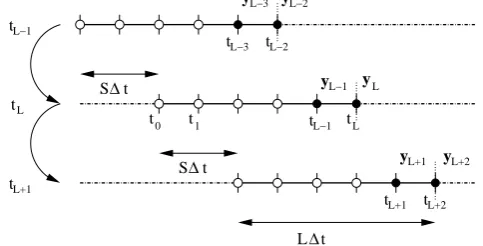
Fig. 1. Chaining of the SDA IEnKS cycles. The schematic
il-lustrates the caseL= 5and a shift ofS= 2time intervals∆tis applied between two updates. The method performs a smoothing update throughout the window but only assimilates the newest ob-servations vectors (that have not been already assimilated) marked by black dots. Note that the time index of the dates and the obser-vations are absolute for this schematic, not relative.
This ensemble attS will form the background for the next analysis.
A typical chaining of the analysis and forecast steps is schematically displayed in Fig. 1. A pseudo-code of the IEnKS is displayed in algorithm 1. It does not show the optional analysis step, since the cycling of data assimilation does not depend on it. It is the same as the one presented in (Bocquet and Sakov, 2013), except that it is here given in the general case1≤S≤Lrather thanS= 1only. It accounts for the possible use of inflation (lines 20,21).
In summary, the IEnKS solves the variational problem of 4D-Var in the ensemble range. Because the variational prob-lem is solved in a reduced space, there is no need for the adjoint evolution and observation models. The IEnKS gen-erates and propagates the posterior perturbations following the scheme of the ensemble Kalman filter. As such, it uses sampled errors of the day.
2.1.2 Single and multiple assimilation of observations
There are some degrees of freedom in the choice ofL,Sand the{βk}1≤k≤L. Let us just mention a few legitimate choices. Firstly, for any choice ofLandS, such that1≤S≤L, the most natural choice for the{βk}1≤k≤Lis to set: βk= 1 fork=L−S+ 1,...L, andβk= 0otherwise. That way, the observations are assimilated once and only once. We call it the single data assimilation scheme (SDA IEnKS). It is sim-ple, and the optional analysis of the update step is merely a forecast of the analyzed state att0, or possibly a forecast of
the full ensemble fromt0. WhenS=L, the DAWs do not
overlap, while they do so ifS < L. The chaining of the data assimilation cycles in the SDA case is displayed in Fig. 1.
For very long data assimilation windows, the use of
multi-ple assimilation (or splitting) of observations, denoted MDA
in the following, can prove numerically efficient (Bocquet
Fig. 1. Chaining of the SDA IEnKS cycles. The schematic
illus-trates the caseL=5 and a shift ofS=2 time intervals1tis ap-plied between two updates. The method performs a smoothing up-date throughout the window but only assimilates the newest obser-vations vectors (that have not been already assimilated) marked by black dots. Note that the time index of the dates and the observations are absolute, not relative, for this schematic.
If the optional analysis step implied forecasting the ensem-ble to or beyondtS, then there is no need to forecast it again.
This ensemble attS will form the background for the next
analysis.
A typical chaining of the analysis and forecast steps is schematically displayed in Fig. 1.
A pseudo-code of the IEnKS is displayed in Algorithm 1. It does not show the optional analysis step, since the cycling of data assimilation does not depend on it. It is the same as the one presented in Bocquet and Sakov (2013), except that here it is given in the general case, 1≤S≤L, rather than the specific case S=1. The pseudo-code accounts for the possible use of inflation (lines 20, 21).
In summary, the IEnKS solves the variational problem of 4D-Var in the ensemble range. Because the variational prob-lem is solved in a reduced space, there is no need for the adjoint evolution and observation models. The IEnKS gen-erates and propagates the posterior perturbations following the scheme of the ensemble Kalman filter. As such, it uses sampled errors of the day.
2.1.2 Single and multiple assimilation of observations
There are some degrees of freedom in the choice ofL,Sand the{βk}1≤k≤L. Let us just mention a few legitimate choices.
Firstly, for any L andS, such that 1≤S≤L, the most natural choice for the{βk}1≤
k≤Lisβk=1 fork=L−S+
1, . . . L, andβk=0 otherwise. That way, the observations are
assimilated once and only once. We call this the single data assimilation scheme (SDA IEnKS). It is simple, and the op-tional analysis of the update step is merely a forecast of the analyzed state att0, or possibly a forecast of the full ensemble
fromt0. WhenS=L, the DAWs do not overlap, but they do
M. Bocquet and P. Sakov: State and parameter estimation with the IEnKS 807
Algorithm 1 A cycle of the lag-L / shift-S / MDA / bundle / Gauss-Newton IEnKS.
Require: tLis present time. Transition modelMk+1←k, observa-tion operatorsHk attk. Algorithm parameters:,e,jmax. E0,
the ensemble att0,yk the observation attk.λis the inflation factor. U is an orthogonal matrix inRN×Nsatisfying U1=1.
βk, 1≤k≤L, are the observation weights within theDAW. 1: j=0,w=0
2: x(00)=E01/N
3: A0=E0−x(00)1T
4: repeat
5: x0=x(00)+A0w
6: E0=x01T+A0
7: fork=1, . . . , Ldo
8: Ek=Mk←k−1(Ek−1)
9: yk=Hk(Ek)1/N 10: Yk=(Hk(Ek)−yk)/ 11: end for
12: ∇Je=(N−1)w− PL
k=1βkYTkR
−1
k (yk−yk) 13: He=(N−1)IN+
PL
k=1βkYTkR
−1 k Yk 14: SolveHe1w= ∇Je
15: w:=w−1w
16: j:=j+1
17: until||1w|| ≤e or j≥jmax
18: E0=x01T+ √
N−1A0He
−1
2U
19: ES=MS←0(E0)
20: xs=ES1/N
21: ES:=xS1T+λ ES−xS1T
For very long data assimilation windows, the use of
multi-ple assimilation (or splitting) of observations, denoted MDA
in the following, can prove numerically efficient (Bocquet and Sakov, 2013). An observation vectory is said to be as-similated with weightβ (0≤β≤1) if the following Gaus-sian observation likelihood is used in the analysis:
p(yβ|x)=e
−β2(y−H (x))TR−1(y−H (x))
p
(2π/β)d|R| , (10)
where|R|is the determinant of R. The upper index ofyβ
refers to the partial assimilation ofywith weightβ. The prior errors attached to the several occurrences of one observation are chosen to be independent. In that light, the{βk}1≤k≤L
are merely the weights of the observation vectors{yk}1≤k≤L
within the DAW. Statistical consistency necessitates that a unique observation vector is assimilated in such a way that the sum of all its weights in the data assimilation experi-ment is 1. For instance, if 1=S≤L, consistency requires thatPL
k=1βk=1. In a more general case in which the
obser-vation vectors have the same number of non-zero weights,L
is a multiple ofS:L=QS, whereQis an integer. As a re-sult, consistency requiresPQ−1
q=0βSq+l=1 withl=1, . . . , S.
In the MDA case (except the SDA subcase) the optional analysis step is more complex since it requires re-weighting
M. Bocquet, P. Sakov: State and parameter estimation with the IEnKS 5
Algorithm 1 A cycle of the lag-L / shift-S / MDA / bundle / Gauss-Newton IEnKS.
Require: tLis present time. Transition modelMk+1←k, observa-tion operatorsHkattk. Algorithm parameters:ǫ,e,jmax.E0,
the ensemble att0,ykthe observation attk. λis the inflation factor.Uis an orthogonal matrix inRN×N
satisfyingU1=1. βk,1≤k≤L, are the observation weights within theDAW. 1: j= 0,w=0
2: x(0)0 =E01/N
3: A0=E0−x(0)0 1T
4: repeat
5: x0=x(0)0 +A0w
6: E0=x01T+ǫA0
7: fork= 1,...,Ldo
8: Ek=Mk←k−1(Ek−1) 9: yk=Hk(Ek)1/N 10: Yk= (Hk(Ek)−yk)/ǫ 11: end for
12: ∇Je= (N−1)w−PLk=1βkYTkR −1
k (yk−yk) 13: He= (N−1)IN+P
L
k=1βkYTkR −1
k Yk 14: SolveHe∆w=∇Je
15: w:=w−∆w 16: j:=j+ 1
17: until||∆w|| ≤e or j≥jmax
18: E0=x01T+√N−1A0He−
1
2U
19: ES=MS←0(E0)
20: xs=ES1/N
21: ES:=xS1T+λ ES−xS1T
and Sakov, 2013). An observation vectoryis said to be as-similated with weightβ(0≤β≤1) if the following Gaussian observation likelihood is used in the analysis:
p(yβ|x) =e
−β2(y−H(x))
TR−1(y−H(x))
p
(2π/β)d|R| , (10)
where |R| is the determinant of R. The upper index of
yβ refers to its partial assimilation with weight β. The prior errors attached to the several occurrences of one ob-servation are chosen to be independent. In that light, the {βk}1≤k≤L are merely the weights of the observation vec-tors{yk}1≤k≤Lwithin theDAW. Statistical consistency im-poses that a unique observation vector is assimilated in such a way that the sum of all its weights in the data assimilation experiment is one. For instance, if1 =S≤L, one requires
PL
k=1βk= 1. In the more general case where the
observa-tion vectors have the same number of non zero weights, then Lis a multiple ofS:L=QS, whereQis an integer. As a re-sult consistency requires:PQq=0−1βSq+l= 1withl= 1,...,S. In the MDA case, except the SDA subcase, the optional analysis step is more complex since it requires to re-weight the observations within theDAWto obtain the correct analy-sis for statest1totLand beyond. More details that are not
directly relevant to this study can be found in (Bocquet and Sakov, 2013).
S∆ S∆
t0 t1 t
t t
t t
t L L−1
L+1
yL
∆ L t
t t t
L+1 L+2 L−2
L−3
t tL−1 L
y
y y
L+2 L+1 L−2
L−3
y yL−1
β β
β β β β
L L
L−1 L−1
L−1
L y
−1
β
yβ1 1
yβ 31 1
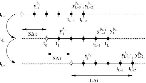
Fig. 2. Chaining of the MDA IEnKS cycles. The schematic
illus-trates the caseL= 5, andS= 2. The method performs a smooth-ing update throughout the window potentially ussmooth-ing all observations within the window (marked by black dots), except for the first ob-servation vector assumed to be already entirely assimilated. Note that the time index for the dates and the observations are absolute for this schematic, not relative.
Note that when the constraintPLk=1βk= 1 is not satis-fied the underlying smoothing probability density function (pdf) will not be the targeted one, but, with well chosen {βk}1≤k≤L, could be a power of it (Bocquet and Sakov, 2013).
These MDA approaches are mathematically consistent in the sense that they are demonstrated to be correct in the lin-ear model, Gaussian statistics case. In (Bocquet and Sakov, 2013), an heuristic argument based on Bayesian ideas justi-fies the use of the method in the nonlinear case.
The chaining of the data assimilation cycles in the MDA case is displayed in Fig. 2. In the experimental Sections 3 and 4, both SDA and MDA schemes will be used.
2.2 Augmented state formalism
We wish to estimate a set of model parametersθ∈RP along with the state variables. To do so, the state space is aug-mented fromx∈RM to a vector
z=
x θ
∈RM+P, (11)
of the joint state and parameter space. From the mathemati-cal point of view the analysis step of the IEnKS is unchanged. As usual in a parameter estimation context, a forward model needs to be introduced for the parameters. For in-stance, it could be the persistence model (θk+1=θk), or some jittering such as a Brownian motion, could be assumed (θk+1=θk+ǫk). Depending on the constraints on the
pa-rameters, this jittering could also be constrained.
Technically, there is nothing more to the joint state and parameter IEnKS than in the state IEnKS. As opposed to the EnKF and EnKS, the objective is not to build covariances to help estimate hidden parameters, but instead to minimize a cost function that depends on the full augmented state. In a
Fig. 2. Chaining of the MDA IEnKS cycles. The schematic
illus-trates the caseL=5, andS=2. The method performs a smooth-ing update throughout the window potentially ussmooth-ing all observations within the window (marked by black dots), except for the first ob-servation vector assumed to be already entirely assimilated. Note that the time index for the dates and the observations are absolute for this schematic, not relative.
the observations within the DAW to obtain the correct anal-yses for statest1totLand beyond. More details that are not
directly relevant to this study can be found in Bocquet and Sakov (2013).
Note that when the constraintPL
k=1βk=1 is not satisfied,
the underlying smoothing probability density function (pdf) will not be the one targeted, but, with well chosen{βk}1≤k≤L, could be a power of it (Bocquet and Sakov, 2013).
These MDA approaches are mathematically consistent in the sense that they are demonstrated to be correct in the lin-ear model, Gaussian statistics case. An heuristic argument based on Bayesian ideas justifies the use of the method in the nonlinear case (Bocquet and Sakov, 2013).
The chaining of the data assimilation cycles in the MDA case is displayed in Fig. 2.
In the experimental Sects. 3 and 4, both SDA and MDA schemes will be used.
2.2 Augmented state formalism
We wish to estimate a set of model parametersθ∈RP along with the state variables. To do so, the state space is aug-mented fromx∈RM to a vector
z=
x θ
∈RM+P, (11)
of the joint state and parameter space. From the mathematical point of view, the analysis step of the IEnKS is unchanged.
As is usual in a parameter estimation context, a forward model needs to be introduced for the parameters. This model could be, for instance, the persistence model (θk+1=θk), or
some jittering such as a Brownian motion, could be assumed (θk+1=θk+k). Depending on the constraints on the
pa-rameters, this jittering could also be constrained.
808 M. Bocquet and P. Sakov: State and parameter estimation with the IEnKS
Technically, there is nothing more in the joint state and parameter IEnKS than in the state IEnKS. As opposed to the EnKF and EnKS, the objective of the joint state and parame-ter IEnKS is not to build covariances to help estimate hidden parameters, but instead to minimize a cost function that de-pends on the full augmented state. In a strongly nonlinear context, this approach could prove superior to the standard EnKF and EnKS.
As mentioned in the introduction, the estimation of model parameters within 4D-Var requires the adjoint model. Be-sides, the computation of the derivative of the cost function with respect to the parameters in terms of the adjoint field can be tedious. Parameter estimation with the IEnKS avoids this time-consuming task.
A potential advantage of the IEnKS over 4D-Var is that the errors of the day are by construction estimated within the IEnKS for all types of variables or parameters, whereas the 4D-Var modeling of background statistics of heterogeneous variables and parameters can be complex (see, for instance, Elbern et al. (2007), relating the modeling of inter-species correlation in a 4D-Var applied to air quality, or Montmerle and Berre (2010) in a meteorological convective scale con-text).
Similarly to state estimation, joint state and parameter es-timation with the IEnKS in theory combines appealing fea-tures of both variational and ensemble Kalman filtering tech-niques. The purpose of the following numerical exploration is to investigate whether this holds true in experiments with low-order models.
3 Numerical experiments with the Lorenz-95 model
The Lorenz-95 one-dimensional model (Lorenz and Em-manuel, 1998) represents a mid-latitude zonal circle of the global atmosphere. It hasM=40 variables{xm}m=1,...,M. Its
dynamics is given by the following set of ordinary differen-tial equations:
dxm
dt =(xm+1−xm−2)xm−1−xm+F , (12)
for m=1, . . . , M, and the domain is periodic (circle-like).
F is chosen to be 8 so that the dynamics is chaotic and has 13 positive Lyapunov exponents. A time step of1t=0.05 is meant to represent a time interval of 6 h in the real atmo-sphere. Unless otherwise stated, the time interval between each observational update will be 1t=0.05, meant to be representative of a data assimilation cycle of global mete-orological models. With such a value for 1t, the data as-similation system is considered weakly nonlinear, leading to statistics of errors weakly diverging from Gaussianity. This model is integrated using the fourth-order Runge–Kutta scheme with a time step of 0.05.
3.1 Setup
Twin experiments are conducted. The truth is represented by a free model run (nature run), meant to be tracked by the data assimilation system. The system is assumed to be fully observed (d=40) every1t, so that Hk=Id, with the
obser-vation error covariance matrix Rk=Id. The related synthetic
observations are generated from the truth, and perturbed ac-cording to the same observation error prior. The performance of a scheme is measured by the temporal mean of a root mean square difference between a state estimate (xa) and the truth (xt). Typically, one averages the following analysis root
mean square error (RMSE):
RMSE=
v u u t
1
M
M X
m=1 xa
m−xmt 2
(13)
over the data assimilation cycles. When this RMSE concerns the system state at present time, i.e., the state at the end of the DAW, we call it the filtering RMSE. When this RMSE con-cerns the state definedL1t in the past, i.e., at the beginning of the DAW, we call it the smoothing RMSE. All data assim-ilation runs will extend over 105cycles after a burn-in period of 5×10³cycles. This guarantees a sufficient convergence of the error statistics.
Unless otherwise stated, the size of the ensemble used with the ensemble methods will beN=20, which is greater than the size of the unstable subspace, and, in the case of this model, makes localization unnecessary.
In this context, we have chosen to implement the infla-tion using the finite-size counterparts of the filters/smoothers (Bocquet et al., 2011). For this model, except in quasi-linear conditions (1t∼0.01), this inflation leads to perfor-mances that are quantitatively very close to the same fil-ter/smoother with optimally tuned uniform inflation (Boc-quet et al., 2011; Boc(Boc-quet and Sakov, 2012). In the following methods like EnKF/IEnKS/EnKS should be understood as EnKF/IEnKS/EnKS with optimally tuned uniform inflation, and will actually be implemented with a single run of the finite-size variants, i.e. EnKF-N/IEnKS-N/EnKS-N, which is much more economical. Any reader not interested in imple-menting the finite-size IEnKS (whose pseudo-code is pre-sented in Algorithm 2), or IEnKS-N, can alternatively op-timally tune the uniform inflation of an EnKF/IEnKS/EnKS to attain very similar results.
3.2 New experiments with the IEnKS
M. Bocquet and P. Sakov: State and parameter estimation with the IEnKS 809
8 M. Bocquet, P. Sakov: State and parameter estimation with the IEnKS
1 5 10 15 20 25 30 35 40 45 50
DAW length L
0.160 0.165 0.170 0.175 0.180 0.185 0.190
0.155 0.200 0.195 0.210 0.220
Filtering analysis RMSE
4D-Var S=1 EnKS-N S=1 SDA IEnKS-N S=1 SDA IEnKS-N S=L MDA IEnKS-N S=1
1 5 10 15 20 25 30 35 40 45 50
DAW length L
0.04 0.05 0.06 0.07 0.08 0.09 0.10 0.12 0.14 0.16 0.18 0.20 0.22
Smoothing analysis RMSE
4D-Var S=1 EnKS-N S=1 SDA IEnKS-N S=1 SDA IEnKS-N S=L MDA IEnKS-N S=1
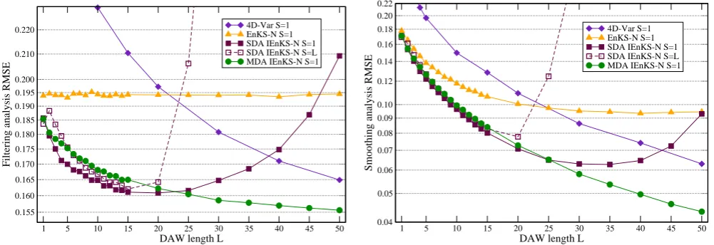
Fig. 3. Comparison of the filtering (left) and smoothing (right) performance of the SDA IEnKS, MDA IEnKS, the EnKS and 4D-Var, in
weakly non-linear conditions corresponding to∆t= 0.05.
1 2 3 4 5 6 7 8 9 10
DAW length L
0.30 0.32 0.34
0.28 0.36
0.29 0.31 0.33 0.35 0.37 0.38 0.39 0.40 0.42 0.44 0.46
0.27
Filtering analysis RMSE
4D-Var S=1 EnKS-N S=1 SDA IEnKS-N S=1 SDA IEnKS-N S=L MDA IEnKS-N S=1
1 2 3 4 5 6 7 8 9 10
DAW length L
0.08 0.10 0.12 0.14 0.16 0.18 0.20 0.22 0.24 0.26 0.28 0.30 0.32 0.34 0.36 0.38 0.40
Smoothing analysis RMSE 4D-Var S=1 EnKS-N S=1 SDA IEnKS-N S=1 SDA IEnKS-N S=L MDA IEnKS-N S=1
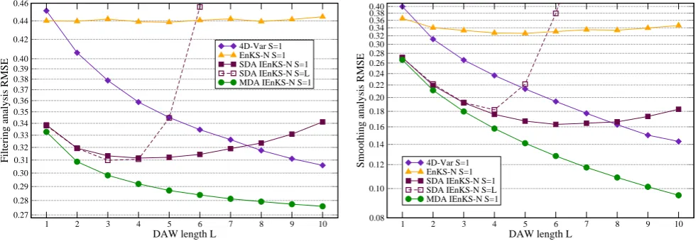
Fig. 4. Comparison of the filtering (left) and smoothing (right) performance of the SDA IEnKS, MDA IEnKS, the EnKS and 4D-Var, in
non-linear conditions corresponding to∆t= 0.20.
– The ensemble Kalman filter (EnKF).
– The ensemble Kalman smoother (EnKS)S= 1.
– The MDA IEnKSS= 1. The {βk}1≤k≤L are chosen
uniform in theDAWand constant in time.
– 4D-Var with S= 1. The background’s magnitude is tuned so as to minimize the global (on all41extended variables)RMSE.
To avoid tuning inflation, the finite-size variants, EnKF-N,
EnKS-N, MDA IEnKS-N, are employed. The DAWlength
is varied in the MDA IEnKS and 4D-Var cases up toL=
50, before a degradation of the performance sets in. In the
EnKS case, theDAWlength is varied up toL= 100, which
corresponds to the optimal performance for the smoothing
estimation ofFby the EnKS.
The forcing parameter is plotted in Fig. 5, over a5×103
-cycle-long segment of the experiment. In the case of the
EnKS, the smoothing estimator forF(at the beginning of the
DAW) is plotted because it is better than the filtering estimate ofF(at the end of theDAW). Because the persistence model is assumed forF, the smoothing and the filtering estimates ofFare the same for the IEnKS and 4D-Var. Because, in ad-dition, the trueFis static, the smoothing and filteringRMSEs should coincide. From Fig. 5, it is clear that the IEnKS sig-nificantly outperforms the EnKF and the EnKS.
The time-averaged analysis root mean square errors (RMSEs) are computed over a much longer run of105cycles.
The scores for the state variables are reported in Fig. 6. The filteringRMSEs (i.e. at present time) of the EnKF or of the
EnKS for anyLare, by construction, the same. The
estima-tion of the forcingF is good enough so that the performance is indistinguishable from the EnKF performance in the case
where F= 8is known. Nevertheless, even in this weakly
nonlinear regime, the IEnKS withL≥1outperforms them.
Confirming the results of Bocquet and Sakov (2013), the gap Fig. 3. Comparison of the filtering (left) and smoothing (right) performance of the SDA IEnKS, MDA IEnKS, the EnKS and 4D-Var, in
weakly nonlinear conditions corresponding to1t=0.05.
Algorithm 2 A cycle of the lag-L / shift-S / MDA / bundle / Gauss-Newton IEnKS-N. Same as algorithm 1 with the ex-ception of the following lines:
Require: Same requirements as algorithm 1.εN=1. 12: ∇Je=N w
εN+wTw
−PL
k=1βkYTkR
−1
k (yk−yk)
18: He=N
εN+wTw
IN−2wwT
(εN+wTw)2
+PL
k=1βkYTkR−k1Yk
19: E0=x01T+ √
N−1A0He− 1 2U 20: ES=MS←0(E0)
21:
– The SDA IEnKS,S=1.
– The MDA IEnKS,S=1. The{βk}1≤k≤Lare chosen to
be uniform in the DAW and constant in time.
– The SDA IEnKS, with S equal to the length of the DAWS=L, so that the DAWs do not overlap. This approach is meant to be computationally economical, and is much more economical than the quasi-static caseS=1, since there is no overlapping of DAWs. – The standard ensemble Kalman smoother (EnKS),
withS=1. The standard ensemble Kalman smoother has been defined in Evensen and van Leeuwen (2000); Evensen (2003, 2009); Cosme et al. (2012).
– 4D-Var with a shiftS=1, corresponding to overlap-ping DAWs and quasi-static conditions. The gradient is obtained by finite differences, which is affordable and precise enough in this small dimensional context. The performance of 4D-Var strongly depends on the back-ground statistics. Since the correlations in the Lorenz-95 system are rather short-ranged, the B-matrix is cho-sen diagonal. The performance of 4D-Var does not
vary much if we introduce some correlation and off-diagonal terms. However, the scaling of the B-matrix is crucial in this context (Kalnay et al., 2007). The longer the DAW is, the smaller the scaling factor should be, since the first guess becomes more accurate. For each experiment, we tuned this scaling so as to obtain the best filtering analysis RMSE.
To avoid tuning inflation, the finite-size variants of the filters and smoothers are employed (SDA IEnKS-N, MDA IEnKS-N, EnKS-N). All EnKF and EnKS, and their finite-size variants in this article are based on the ensemble trans-form square root Kalman filter (Bishop et al., 2001; Hunt et al., 2007; Bocquet et al., 2011). These five data assim-ilation systems are compared in weakly nonlinear condi-tions (1t=0.05) chosen to roughly represent synoptic scale meteorology dynamics (Lorenz and Emmanuel, 1998), and more nonlinear conditions (1t=0.20 between updates). The time-averaged analysis RMSE is plotted in Fig. 3 for the for-mer case, and in Fig. 4 for the latter case, as a function of the length of the DAW.
Let us first notice that the filtering performance of the EnKS is, by construction, given by that of the EnKF, what-ever the length of the DAWs. This explains why the filtering RMSE of EnKS is constant, modulo statistical noise. When comparing the filtering performances of the EnKF/EnKS and 4D-Var, the conclusions of Kalnay et al. (2007) are rein-forced. 4D-Var does not perform as well for short DAWs and performs better for long DAWs. In addition, we note that the same conclusion applies to the smoothing performance, even though the crossover point might be different.
Considering filtering as well as smoothing, the MDA IEnKS S=1 significantly outperforms 4D-Var and the EnKF/EnKS in all regimes. The SDA IEnKS S=1, also performs very well, but its performance wanes with longer DAWs, which is why the MDA IEnKS was introduced by
810 M. Bocquet and P. Sakov: State and parameter estimation with the IEnKS
8 M. Bocquet, P. Sakov: State and parameter estimation with the IEnKS
1 5 10 15 20 25 30 35 40 45 50
DAW length L
0.160 0.165 0.170 0.175 0.180 0.185 0.190
0.155 0.200 0.195 0.210 0.220
Filtering analysis RMSE
4D-Var S=1 EnKS-N S=1 SDA IEnKS-N S=1 SDA IEnKS-N S=L MDA IEnKS-N S=1
1 5 10 15 20 25 30 35 40 45 50
DAW length L
0.04 0.05 0.06 0.07 0.08 0.09 0.10 0.12 0.14 0.16 0.18 0.20 0.22
Smoothing analysis RMSE
4D-Var S=1 EnKS-N S=1 SDA IEnKS-N S=1 SDA IEnKS-N S=L MDA IEnKS-N S=1
Fig. 3. Comparison of the filtering (left) and smoothing (right) performance of the SDA IEnKS, MDA IEnKS, the EnKS and 4D-Var, in
weakly non-linear conditions corresponding to∆t= 0.05.
1 2 3 4 5 6 7 8 9 10
DAW length L
0.30 0.32 0.34
0.28 0.36
0.29 0.31 0.33 0.35 0.37 0.38 0.39 0.40 0.42 0.44 0.46
0.27
Filtering analysis RMSE
4D-Var S=1 EnKS-N S=1 SDA IEnKS-N S=1 SDA IEnKS-N S=L MDA IEnKS-N S=1
1 2 3 4 5 6 7 8 9 10
DAW length L
0.08 0.10 0.12 0.14 0.16 0.18 0.20 0.22 0.24 0.26 0.28 0.30 0.32 0.34 0.36 0.38 0.40
Smoothing analysis RMSE 4D-Var S=1 EnKS-N S=1 SDA IEnKS-N S=1 SDA IEnKS-N S=L MDA IEnKS-N S=1
Fig. 4. Comparison of the filtering (left) and smoothing (right) performance of the SDA IEnKS, MDA IEnKS, the EnKS and 4D-Var, in
non-linear conditions corresponding to∆t= 0.20.
– The ensemble Kalman filter (EnKF).
– The ensemble Kalman smoother (EnKS)S= 1. – The MDA IEnKSS= 1. The{βk}1≤k≤L are chosen
uniform in theDAWand constant in time.
– 4D-Var with S= 1. The background’s magnitude is tuned so as to minimize the global (on all41extended variables)RMSE.
To avoid tuning inflation, the finite-size variants, EnKF-N, EnKS-N, MDA IEnKS-N, are employed. TheDAW length is varied in the MDA IEnKS and 4D-Var cases up to L= 50, before a degradation of the performance sets in. In the EnKS case, theDAWlength is varied up toL= 100, which corresponds to the optimal performance for the smoothing estimation ofF by the EnKS.
The forcing parameter is plotted in Fig. 5, over a5×103
-cycle-long segment of the experiment. In the case of the
EnKS, the smoothing estimator forF(at the beginning of the
DAW) is plotted because it is better than the filtering estimate
ofF(at the end of theDAW). Because the persistence model is assumed forF, the smoothing and the filtering estimates ofFare the same for the IEnKS and 4D-Var. Because, in ad-dition, the trueFis static, the smoothing and filteringRMSEs should coincide. From Fig. 5, it is clear that the IEnKS sig-nificantly outperforms the EnKF and the EnKS.
The time-averaged analysis root mean square errors (RMSEs) are computed over a much longer run of105cycles.
The scores for the state variables are reported in Fig. 6. The filteringRMSEs (i.e. at present time) of the EnKF or of the EnKS for anyLare, by construction, the same. The estima-tion of the forcingFis good enough so that the performance is indistinguishable from the EnKF performance in the case whereF= 8 is known. Nevertheless, even in this weakly nonlinear regime, the IEnKS withL≥1outperforms them. Confirming the results of Bocquet and Sakov (2013), the gap
Fig. 4. Comparison of the filtering (left) and smoothing (right) performance of the SDA IEnKS, MDA IEnKS, the EnKS and 4D-Var, in
nonlinear conditions corresponding to1t=0.20.
Bocquet and Sakov (2013). For very short DAWs (L=1,2 in the case1t=0.05), the performances of the SDA IEnKS
S=1 and MDA IEnKSS=1 are equal (L=1) or very close (L=2). For intermediate DAW lengths, the SDA IEnKS
S=1 can slightly outperform MDA IEnKSS=1. This is not surprising, since the SDA IEnKS algorithm is meant to be optimal for sufficiently short DAWs, whereas the MDA IEnKS algorithm is only guaranteed to be optimal in lin-ear/Gaussian conditions.
Practically, in weakly nonlinear conditions (1t=0.05), the IEnKSS=1 only requires one to two propagations of the ensemble within the DAW. Consistently, it was shown in Bocquet and Sakov (2013) that a linearized variant of the algorithm, requiring one propagation of the ensemble within the DAW to compute the sensitivity, performed just as well in these conditions. It is nevertheless tempting to check whether this cost can be reduced by using non-overlapping windows
S=L, and performing the analysis everyL1t. This would divide the cost of model runs byL, but this effect might nev-ertheless be offset by an higher number of iterations required for the analysis.
Quite surprisingly, the SDA IEnKSS=Lperforms very well for DAWs of length smaller than 0.80 (about twice the doubling time of the Lorenz-95 model). It is useless beyond that length, which was to be expected since the background at the beginning of the DAW results from a long forecast within the DAW, as opposed to a forecast of only1t in the quasi-staticS=1 case.
In stronger nonlinear conditions, the variational methods (4D-Var and IEnKS) easily outperform the EnKF/EnKS. In particular, 4D-Var outperforms the EnKF/EnKS as soon as the the DAW reachesL=2.
3.3 Joint state and forcingFestimation
A twin experiment is conducted in a situation where F is unknown. The true model (nature run) has forcing F =8. The model used for assimilation and forecast has the initial valueF =7.
In addition to the state variables, the forcing parameterF
will be estimated as well. Hence, the state vector x∈RM withM=40 will be extended to the joint vector of sizeM+
P =41, with its 41st entry being the forcing parameter. The persistence model will be assumed for the evolution of the model parameter.
Because the filters and smoothers used here are all deter-ministic, the only source of stochasticity to generate the vari-ability inF comes from the initialization of the ensemble. The forcing parameter of a member is initialized to 7+ε, whereεis independently drawn from a normal distribution of standard deviation 0.1. The augmented state IEnKS will be compared to several augmented state alternatives. Specif-ically, we shall consider in this experiment:
– The ensemble Kalman filter (EnKF).
– The ensemble Kalman smoother (EnKS)S=1. – The MDA IEnKSS=1. The{βk}1≤k≤Lare chosen to
be uniform in the DAW and constant in time.
– 4D-Var with S=1. The background’s magnitude is tuned so as to minimize the global (on all 41 extended variables) RMSE.
M. Bocquet and P. Sakov: State and parameter estimation with the IEnKS 811
M. Bocquet, P. Sakov: State and parameter estimation with the IEnKS 9
0 1000 2000 3000 4000 5000
Time 8.10 8.05 8 7.95 7.90
Analysis of parameter F
EnKF-N EnKS-N L=50 IEnKF-N IEnKS-N L=5 IEnKS-N L=10 IEnKS-N L=30
Fig. 5. Plot of the Lorenz ’95 forcing parameterF as a function of the cycle index of the data assimilation experiment. F is es-timated by several filters and smoothers with an ensemble of size N= 20. The forcing of the true model isF= 8. The MDA IEnKS for L= 1,5,10 and30 is compared to the EnKF and the EnKS (L= 50). The finite-size variants of these methods are used: they do not require inflation and perform, in this context, as well as with optimally tuned inflation.
0 1 5 10 20 30 50
Data assimilation window length (in ∆t) 0.25 0.05 0.10 0.15 0.07 0.125 0.20 0.30
Analysis RMSE (state variables)
4D-Var filtering 4D-Var smoothing EnKF-N/EnKS-N filtering EnKS-N smoothing MDA IEnKS-N filtering MDA IEnKS-N smoothing
Fig. 6. Root mean square errors for the analysis of the state vector
at present time (filtering) or the retrospective analysis of the state vector (smoothing) for the EnKF, EnKS and the IEnKS, in the case of the Lorenz ’95 model, with∆t= 0.05.
in the smoothing performance between the EnKS and the IEnKS significantly increases asLincreases. In this weakly nonlinear regime, the number of iterations required by the IEnKS is close to one, and its performance equals that of the linearized IEnKS (Bocquet and Sakov, 2013).
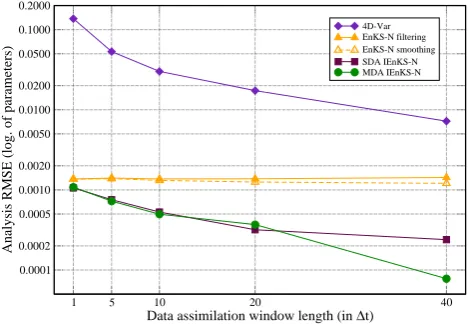
The scores for the estimation of the forcing parameter are reported in Fig. 7. By construction the filtering performance of the EnKF and the EnKS at anyLis the same, about0.018. The parameter smoothingRMSEfor the EnKS is optimal for L∼100and is about0.015. By construction, the analysis at present time and retrospective analysis ofF by the IEnKS
1
1 5 10 20 30 50 100
Data assimilation window length (in ∆t) 0.001 0.002 0.004 0.008 0.016 0.032 0.064 0.128
Analysis RMSE (parameter F) 4D-Var filtering/smoothing EnKF-N/EnKS-N filtering EnKS-N smoothing
MDA IEnKS-N filtering/smoothing
Fig. 7. Root mean square errors for the analysis ofF at present time (filtering) or the retrospective analysis ofF(smoothing) for the EnKF, EnKS and the IEnKS, in the case of the Lorenz ’95 model, with∆t= 0.05.
is the same. Even in the caseL= 1, the so-called iterative ensemble Kalman filter (IEnKF) outranks the EnKS with an
RMSE of0.013. With increasingL, this performance gets better and better and reaches theRMSEof7.5×10−4forL=
50.
The estimation of 4D-Var only gets better than the EnKF forDAWs of lengthL= 50. This counter-performance can only be explained by a poor specification of the error co-variance matrix. Indeed, the scaling of the background error statistics for the state variables should be different from the scaling of the background error statistics for the parameter. However, the separate tuning of scalings requires additional work that the IEnKS does not require. This hypothesis will be checked in Sect. 5.
4 Numerical experiments with a coupled Lorenz ’95 -tracer model
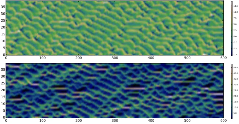
In this section we introduce a simple extension of the Lorenz ’95 model with a tracer field advected by the Lorenz ’95 field representing an advective wind. It is meant to test the ability of the IEnKS for joint state and parameter estimation in the dynamical context of an online atmospheric chemical model, with heterogeneous variables.
4.1 Extending the Lorenz’ 95 model
We shall think of the variablesxmof the Lorenz ’95 as wind speed and direction variables defined on the circle. A tracer fieldcm+1
2, m= 1,...,M= 40will be added to the model variables, for a total of80variables. These variables are
de-Fig. 5. Plot of the Lorenz-95 forcing parameterF as a function of the cycle index of the data assimilation experiment.F is esti-mated by several filters and smoothers with an ensemble of size
N=20. The forcing of the true model isF=8. The MDA IEnKS forL=1,5,10 and 30 is compared to the EnKF and the EnKS (L=50). The finite-size variants of these methods are used: they do not require inflation and perform in this context as well as with optimally tuned inflation.
corresponds to the optimal performance for the smoothing estimation ofF by the EnKS.
The forcing parameter is plotted in Fig. 5, over a 5×10³ -cycle-long segment of the experiment. In the case of the EnKS, the smoothing estimator forF (at the beginning of the DAW) is plotted because it is better than the filtering estimate ofF(at the end of the DAW). Because the persistence model is assumed forF, the smoothing and the filtering estimates of F are the same for the IEnKS and 4D-Var. In addition, because the trueF is static, the smoothing and filtering RM-SEs should coincide. From Fig. 5, it is clear that the IEnKS significantly outperforms the EnKF and the EnKS.
The time-averaged analysis root mean square errors (RM-SEs) are computed over a much longer run of 105cycles. The scores for the state variables are reported in Fig. 6. The filter-ing RMSEs (i.e., the RMSEs at present time) of the EnKF or of the EnKS for anyL are, by construction, the same. The estimation of the forcingF is good enough that the per-formance is indistinguishable from the EnKF perper-formance whenF =8 is known. Nevertheless, even in this weakly non-linear regime, the IEnKS withL≥1 outperforms the EnKF and EnKS. Confirming the results of Bocquet and Sakov (2013), the gap in the smoothing performance between the EnKS and the IEnKS significantly increases asLincreases. In this weakly nonlinear regime, the number of iterations re-quired by the IEnKS is close to one, and its performance equals that of the linearized IEnKS (Bocquet and Sakov, 2013).
The scores for the estimation of the forcing parameter are reported in Fig. 7. By construction, the filtering performance
M. Bocquet, P. Sakov: State and parameter estimation with the IEnKS 9
0 1000 2000 3000 4000 5000
Time 8.10 8.05 8 7.95 7.90
Analysis of parameter F
EnKF-N EnKS-N L=50 IEnKF-N IEnKS-N L=5 IEnKS-N L=10 IEnKS-N L=30
Fig. 5. Plot of the Lorenz ’95 forcing parameterF as a function of the cycle index of the data assimilation experiment. F is es-timated by several filters and smoothers with an ensemble of size N= 20. The forcing of the true model isF= 8. The MDA IEnKS for L= 1,5,10 and 30is compared to the EnKF and the EnKS (L= 50). The finite-size variants of these methods are used: they do not require inflation and perform, in this context, as well as with optimally tuned inflation.
0 1 5 10 20 30 50
Data assimilation window length (in ∆t) 0.25 0.05 0.10 0.15 0.07 0.125 0.20 0.30
Analysis RMSE (state variables)
4D-Var filtering 4D-Var smoothing EnKF-N/EnKS-N filtering EnKS-N smoothing MDA IEnKS-N filtering MDA IEnKS-N smoothing
Fig. 6. Root mean square errors for the analysis of the state vector
at present time (filtering) or the retrospective analysis of the state vector (smoothing) for the EnKF, EnKS and the IEnKS, in the case of the Lorenz ’95 model, with∆t= 0.05.
in the smoothing performance between the EnKS and the IEnKS significantly increases asLincreases. In this weakly nonlinear regime, the number of iterations required by the IEnKS is close to one, and its performance equals that of the linearized IEnKS (Bocquet and Sakov, 2013).
The scores for the estimation of the forcing parameter are reported in Fig. 7. By construction the filtering performance of the EnKF and the EnKS at anyLis the same, about0.018. The parameter smoothingRMSEfor the EnKS is optimal for L∼100and is about0.015. By construction, the analysis at present time and retrospective analysis ofF by the IEnKS
1
1 5 10 20 30 50 100
Data assimilation window length (in ∆t) 0.001 0.002 0.004 0.008 0.016 0.032 0.064 0.128
Analysis RMSE (parameter F) 4D-Var filtering/smoothing EnKF-N/EnKS-N filtering EnKS-N smoothing
MDA IEnKS-N filtering/smoothing
Fig. 7. Root mean square errors for the analysis ofF at present time (filtering) or the retrospective analysis ofF(smoothing) for the EnKF, EnKS and the IEnKS, in the case of the Lorenz ’95 model, with∆t= 0.05.
is the same. Even in the caseL= 1, the so-called iterative ensemble Kalman filter (IEnKF) outranks the EnKS with an
RMSE of0.013. With increasingL, this performance gets better and better and reaches theRMSEof7.5×10−4forL=
50.
The estimation of 4D-Var only gets better than the EnKF forDAWs of lengthL= 50. This counter-performance can only be explained by a poor specification of the error co-variance matrix. Indeed, the scaling of the background error statistics for the state variables should be different from the scaling of the background error statistics for the parameter. However, the separate tuning of scalings requires additional work that the IEnKS does not require. This hypothesis will be checked in Sect. 5.
4 Numerical experiments with a coupled Lorenz ’95 -tracer model
In this section we introduce a simple extension of the Lorenz ’95 model with a tracer field advected by the Lorenz ’95 field representing an advective wind. It is meant to test the ability of the IEnKS for joint state and parameter estimation in the dynamical context of an online atmospheric chemical model, with heterogeneous variables.
4.1 Extending the Lorenz’ 95 model
We shall think of the variablesxmof the Lorenz ’95 as wind speed and direction variables defined on the circle. A tracer fieldcm+1
2,m= 1,...,M= 40will be added to the model variables, for a total of80variables. These variables are
de-Fig. 6. Root mean square errors for the analysis of the state vector
at present time (filtering) or the retrospective analysis of the state vector (smoothing) for the EnKF, EnKS and the IEnKS, in the case of the Lorenz-95 model, with1t=0.05.
M. Bocquet, P. Sakov: State and parameter estimation with the IEnKS 9
0 1000 2000 3000 4000 5000
Time 8.10 8.05 8 7.95 7.90
Analysis of parameter F
EnKF-N EnKS-N L=50 IEnKF-N IEnKS-N L=5 IEnKS-N L=10 IEnKS-N L=30
Fig. 5. Plot of the Lorenz ’95 forcing parameterF as a function of the cycle index of the data assimilation experiment. F is es-timated by several filters and smoothers with an ensemble of size N= 20. The forcing of the true model isF= 8. The MDA IEnKS for L= 1,5,10 and30 is compared to the EnKF and the EnKS (L= 50). The finite-size variants of these methods are used: they do not require inflation and perform, in this context, as well as with optimally tuned inflation.
0 1 5 10 20 30 50
Data assimilation window length (in ∆t) 0.25 0.05 0.10 0.15 0.07 0.125 0.20 0.30
Analysis RMSE (state variables)
4D-Var filtering 4D-Var smoothing EnKF-N/EnKS-N filtering EnKS-N smoothing MDA IEnKS-N filtering MDA IEnKS-N smoothing
Fig. 6. Root mean square errors for the analysis of the state vector
at present time (filtering) or the retrospective analysis of the state vector (smoothing) for the EnKF, EnKS and the IEnKS, in the case of the Lorenz ’95 model, with∆t= 0.05.
in the smoothing performance between the EnKS and the IEnKS significantly increases asLincreases. In this weakly nonlinear regime, the number of iterations required by the IEnKS is close to one, and its performance equals that of the linearized IEnKS (Bocquet and Sakov, 2013).
The scores for the estimation of the forcing parameter are reported in Fig. 7. By construction the filtering performance of the EnKF and the EnKS at anyLis the same, about0.018. The parameter smoothingRMSEfor the EnKS is optimal for L∼100and is about0.015. By construction, the analysis at present time and retrospective analysis ofF by the IEnKS
1
1 5 10 20 30 50 100
Data assimilation window length (in ∆t) 0.001 0.002 0.004 0.008 0.016 0.032 0.064 0.128
Analysis RMSE (parameter F) 4D-Var filtering/smoothing EnKF-N/EnKS-N filtering EnKS-N smoothing
MDA IEnKS-N filtering/smoothing
Fig. 7. Root mean square errors for the analysis ofF at present time (filtering) or the retrospective analysis ofF(smoothing) for the EnKF, EnKS and the IEnKS, in the case of the Lorenz ’95 model, with∆t= 0.05.
is the same. Even in the caseL= 1, the so-called iterative ensemble Kalman filter (IEnKF) outranks the EnKS with an
RMSE of 0.013. With increasing L, this performance gets better and better and reaches theRMSEof7.5×10−4forL=
50.
The estimation of 4D-Var only gets better than the EnKF forDAWs of lengthL= 50. This counter-performance can only be explained by a poor specification of the error co-variance matrix. Indeed, the scaling of the background error statistics for the state variables should be different from the scaling of the background error statistics for the parameter. However, the separate tuning of scalings requires additional work that the IEnKS does not require. This hypothesis will be checked in Sect. 5.
4 Numerical experiments with a coupled Lorenz ’95 -tracer model
In this section we introduce a simple extension of the Lorenz ’95 model with a tracer field advected by the Lorenz ’95 field representing an advective wind. It is meant to test the ability of the IEnKS for joint state and parameter estimation in the dynamical context of an online atmospheric chemical model, with heterogeneous variables.
4.1 Extending the Lorenz’ 95 model
We shall think of the variablesxmof the Lorenz ’95 as wind speed and direction variables defined on the circle. A tracer fieldcm+1
2,m= 1,...,M= 40will be added to the model variables, for a total of80variables. These variables are
de-Fig. 7. Root mean square errors for the analysis ofF at present time (filtering) or the retrospective analysis ofF (smoothing) for the EnKF, EnKS and the IEnKS, in the case of the Lorenz-95 model, with1t=0.05.
of the EnKF and the EnKS at anyL is the same, approxi-mately 0.018. The parameter smoothing RMSE for the EnKS is approximately 0.015 and is optimal forL∼100. By con-struction, the analysis at present time and retrospective anal-ysis ofF by the IEnKS is the same. Even in the caseL=1, the so-called iterative ensemble Kalman filter (IEnKF) out-performs the EnKS with an RMSE of 0.013. With increasing
L, this performance improves more and more, reaching the RMSE of 7.5×10⁻⁴forL=50.
The estimation of 4D-Var only becomes better than that of the EnKF for DAWs of length L=50. This counter-performance can only be explained by a poor specification of the error covariance matrix. Indeed, the scaling of the background error statistics for the state variables should be