www.theoryofcomputing.org
Randomized Polynomial-Time Identity
Testing for Noncommutative Circuits
Vikraman Arvind
Pushkar S. Joglekar
Partha Mukhopadhyay
S. Raja
∗Received August 13, 2017; Revised October 4, 2018; Published October 13, 2019
Abstract: In this paper we show that black-box polynomial identity testing (PIT) for n -variate noncommutative polynomials f of degreeDwith at mosttnonzero monomials can be done in randomizedpoly(n,logt,logD)time, and consequently in randomizedpoly(n,logt,s)
time if f is computable by a circuit of sizes. This result makes progress on a question that has been open for over a decade. Our algorithm is based on efficiently isolating a monomial using nondeterministic automata.
The above result does not yield an efficient randomized PIT for noncommutative circuits in general, as noncommutative circuits of sizescan compute polynomials with a double-exponential (ins) number of monomials. As a first step, we consider a natural class of homogeneous noncommutative circuits, that we call+-regular circuits, and give awhite-box
polynomial-time deterministic PIT for them. These circuits can compute noncommutative polynomials with number of monomials double-exponential in the circuit size. Our algorithm combines some new structural results for +-regular circuits with known PIT results for noncommutative algebraic branching programs, a rank bound for commutative depth-3
A preliminary version of this paper appeared in the Proceedings of the 49th ACM Symp. on Theory of Computing (STOC’17) [4].
∗Part of the work was done while the author was a postdoctoral fellow at Chennai Mathematical Institute, India.
ACM Classification:F.1.2
AMS Classification:68W20
identities, and an equivalence testing problem for words. Finally, we solve theblack-box
PIT problem for depth-3+-regular circuits in randomized polynomial time. In particular, we show if f is a nonzero noncommutative polynomial innvariables over the fieldFcomputed
by a depth-3+-regular circuit of sizes, then fcannot be a polynomial identity for the matrix algebraMs(F)whenFis sufficiently large depending on the degree of f.
1
Introduction
Noncommutative computation, introduced in complexity theory by Hyafil [12] and Nisan [19], is a central field of algebraic complexity theory. The main algebraic structure of interest is the free noncommutative ringFhZiover a fieldF, whereZ={z1,z2, . . . ,zn},zi,1≤i≤nare free noncommuting variables.1
A fundamental problem in the subject is designing efficient algorithms for noncommutative Polyno-mial Identity Testing. The problem can be stated as follows:
Let f∈FhZibe a polynomial represented by a noncommutative arithmetic circuitC. The polynomial
f can be either given by a black-box forC(using which we can evaluate the polynomial f on matrices with entries fromFor an extension field), or the circuitCmay be explicitly given. The algorithmic
problem is to check if the polynomial computed byCis identically zero. We recall the formal definition of a noncommutative arithmetic circuit.
Definition 1.1. Anoncommutative arithmetic circuit Cover a fieldFand indeterminatesz1,z2, . . . ,znis
a directed acyclic graph (DAG) with each node of indegree zero labeled by a variable or a scalar constant fromF: the indegree 0 nodes are the input nodes of the circuit. Each internal node of the DAG is of
indegree two and is labeled by either a+or a×(indicating that it is a plus gate or multiplication gate, respectively). Furthermore, the two inputs to each×gate are designated as left and right inputs which is the order in which the gate multiplication is done. A gate ofCis designated asoutput. Each internal gate computes a polynomial (by adding or multiplying its input polynomials), where the polynomial computed at an input node is just its label. Thepolynomial computedby the circuit is the polynomial computed at its output gate. An arithmetic circuit is a formula if the fan-out of every gate is at most one.
Notice that if the size of circuitCissthen the degree of the polynomial computed byCcan be 2s. Bogdanov and Wee [8] have shown a randomized polynomial-time algorithm when the degree of the noncommutative circuitCis polynomially bounded insandn. Their algorithm is based on a classical result of Amitsur-Levitzki [3] stated below.
Theorem 1.2 (Amitsur-Levitzki Theorem). For any fieldF, a nonzero noncommutative polynomial
P∈FhZiof degree≤2d−1is not a polynomial identity for the matrix algebraMd(F). That is to say, P
does not vanish on all d×d matrices overF.
Remark 1.3. There is a second part to the Amitsur-Levitzki theorem which states thatMd(F)has degree
2didentities. In particular, thestandard polynomialS2d(x1, . . . ,x2d) =∑σ∈S2dsgn(σ)xσ(1)· · ·xσ(2d), is a
minimal identity forMd(F).
1Thez
Bogdanov and Wee’s randomized PIT algorithm [8] applies the above theorem to obtain a randomized PIT as follows: LetC(z1,z2, . . . ,zn)be a circuit of syntactic degree bounded by 2d−1. For eachi∈[n], substitute the variableziby ad×dmatrixMiof commuting indeterminates. More precisely, the(`,k) -th entry ofMi isz(`,i)k where 1≤`,k≤d. ByTheorem 1.2, the matrixMf = f(M1,M2, . . . ,Mn)is not identically zero. Hence, inMf there is an entry(`0,k0)which has thecommutativenonzero polynomial g`0,k0 over the variables{z(i)
`,k: 1≤i≤n,1≤`,k≤d}. Notice that the degree of the polynomialg`0,k0 is at
most 2d−1. If we do random substitutions from an extension field ofFof size at least 4d, then we get a
randomized polynomial identity testing algorithm, with error probability at most 1/2, by thePolynomial Identity Lemma2[20,26,18,9,27,28].
The problem with this approach for general noncommutative circuits (whose degree can be 2s) is that the dimension of the matrices grows linearly with the degree of the polynomial. Therefore, this approach only yields a randomized exponential-time algorithm for the problem. Finding an efficient randomized identity test for general noncommutative circuits is a well-known open problem, as mentioned in a recent workshop on algebraic complexity theory (WACT 2016).
We also recall the definition of noncommutative algebraic branching programs [23].
Definition 1.4. A homogeneousnoncommutative algebraic branching programABP is a layered DAG with one in-degree zero source nodes, and one out-degree zero sink nodet. The vertices are partitioned into layers 0,1, . . . ,d (source at layer 0 and sink at layerd). Edges go only from layerito layeri+1 for eachi≤d−1. Each edge is labeled with a homogeneous linear form in the noncommuting variables
{xi|1≤i≤n}. For eachs-to-tdirected pathγ =e1,e2, . . . ,ed, let fγ =`1·`2· · ·`d be the product of
the linear forms`i labeling the edges in that order. The ABP computes the homogeneous degreed
noncommutative polynomial f =∑γ fγ∈FhXi, where the sum is over all directed pathsγfromstot.
We note that Raz and Shpilka [23] have shown a white-box deterministic polynomial-time PIT for noncommutative ABPs. Forbes-Shpilka [11] and Agrawal et al. [1] have given a quasi-polynomial-time black-box algorithm for small degree noncommutative ABPs.
2
Main results
The main result of the paper is the following theorem that we show about noncommutative identities which is of independent mathematical interest.
Theorem 2.1. LetFbe a field of size more than(n+2)d. Let f∈Fhz1,z2, . . . ,znibe a nonzero polynomial of degree d and with t nonzero monomials. Then f cannot be a polynomial identity for the matrix ring Mk(F)for k≥ dlogte+1.
The above theorem yields a randomized PIT forblack-boxnoncommutative polynomials. To see this, suppose f∈Fhz1,z2, . . . ,znibe a nonzero polynomial of degreedand withtnonzero monomials. We can
assumeFis of size more than(n+2)d (if required, we take a suitable extension field). If f 6≡0 then, by Theorem 2.1, the polynomial f does not vanish if we substitute for eachzi,(logt+1)×(logt+1)matrices
of distinct commuting indeterminates. Indeed, f will evaluate to a nonzero(logt+1)×(logt+1)matrix whose entries are polynomials in commuting variables of degree at mostd. For any nonzero entry of this matrix, by applying the Polynomial Identity Lemma (Lemma 3.3) for commutative polynomials, random substitution fromF(or a suitable extension field) for the commuting variables is nonzero with
high probability.
Corollary 2.2. Let f ∈Fhz1,z2, . . . ,znibe a noncommutative polynomial of degree d and sparsity t given
by a black-box, where the black-box can be evaluated on matrices overFor an extension field. Then
there is a randomized algorithm to check whether f is an identically zero polynomial that runs in time poly(logd,n,logt).
In particular, suppose C is a noncommutative arithmetic circuit, given by black-box access, of size s computing a polynomial in n variables of sparsity t. There is a randomized algorithm that checks if
C≡0in timepoly(s,n,logt).
To second part of the corollary follows becauseCcomputes a polynomial of degree bounded by 2s.
Remark 2.3.
1. It is interesting to compareTheorem 2.1with the classical Amitsur-Levitski theorem. Our result brings out the importance of the number of monomials in a polynomial identity ford×d matrices. It implies that any polynomial identity f ford×dmatrices over a fieldFof size more than degf
must have more than 2d−1monomials.
2. We also note that the dimensionkof the matrix ringMk(F)inTheorem 2.1is nearly optimal up
to a logarithmic factor. In fact, the second part of the Amitsur-Levitzki theorem states that the standard polynomialS2d(x1, . . . ,x2d), is a minimal identity forMd(F). Notice that the number of
monomials in the standard polynomial is 2O(dlogd).
In general, a noncommutative circuit of sizescan compute a polynomial that can have 22Ω(s) mono-mials. For example the polynomial f(x,y) = (x+y)2s has noncommutative circuit of sizeO(s)but the number of monomials is 22s. We consider identity testing for a subclass of homogeneous noncommutative circuits, that we call+-regular circuits. These are syntactic homogeneous circuits where the+gates can be partitioned intolayerssuch that the following holds:
(i) There are no directed paths between the+gates within a layer.
(ii) All+gates in a layer have the same syntactic degree.
(iii) The output gate is a+gate.
(iv) All input to output paths go through exactly one+gate in each layer.
The+-depthof a+-regular circuit is the number of+-layers in it. A couple of remarks about+-regular circuits are in order.
• We note that the computational power of noncommutative+-regular circuits is quite limited. We can easily adapt Nisan’s rank-based argument [19] to show that the noncommutative permanent cannot be computed by polynomial-size+-regular circuits. Such a result is not known for general noncommutative circuits.
• However, polynomial-size+-regular circuits of+-depth 2 can compute polynomials of exponential degree and a double-exponential number of monomials. Such polynomials cannot be computed by bounded-depth noncommutative circuits.
• As is evident from the example (x+y)2s, notice that+-regular circuits of sizescan compute polynomials of degree 2swith 22Ω(s) monomials. Nevertheless, we are able to exploit the circuit’s structure to give a deterministic polynomial-time identity testing algorithm for such circuits.
Theorem 2.5. Let C be a noncommutative+-regular circuit of size s given as a white-box computing a
polynomial inFhXi. There is a deterministic polynomial-time algorithm that tests whether C computes
the identically zero polynomial.
Finally, we give a randomized polynomial identity test for+-regular circuits of+-depth 2 in the black-box model. We denote such circuits byΣΠ∗Σ.
Remark 2.6. We use this notation because the polynomials computed byΣΠ∗Σare sums of products of
linear forms, like the well-studiedΣΠΣcircuits. Our notation also brings out their+-regular structure:
there are two+-layers. The top+gate is the output gate and the bottom+-layer consists of gates computing homogeneous linear forms. TheΠ∗indicates that between the two+-layers we can have
several×gates. However,+-regularity guarantees that all inputs to the top+gate have the same syntactic degree.
Theorem 2.7. LetFbe a field of size more than D. Let f(x1, . . . ,xn)∈FhXibe a nonzero homogeneous
polynomial of degree D computed by aΣΠ∗Σcircuit with top gate fan-in s and the fan-in of the product
gates are D. Then f cannot be a polynomial identity for the matrix ringMs(F).
Theblack-boxrandomized polynomial identity test forΣΠ∗Σarithmetic circuits is an immediate
corollary.
Corollary 2.8. Let C be a depth-three+-regular circuit of size s computing a polynomial f(x1, . . . ,xn)∈
FhXi, where the circuit C is given only by black-box access. Then, there is a randomized algorithm that
checks whether f is identically zero, and the algorithm runs in timepoly(s,n).
2.1 Outline of the proofs
In this section, we give informal description of the proofs forTheorem 2.1,Theorem 2.5, andTheorem 2.7.
Black-box algorithm for noncommutative polynomials of exponential sparsity
{z1,z2, . . . ,zn}, and the polynomial f is anF-linear combination of monomials. Degreedmonomials are
elements of{z1,z2, . . . ,zn}d. Letmbe a degree-dmonomial. We use the notationm[i]to denote thei-th variable in the monomial. More precisely, ifm=zj1zj2· · ·zji−1zji· · ·zjd thenm[i] =zji.
Converting to a bivariate polynomial
It is convenient to convert, by a simple encoding trick, the given noncommutative polynomial into a noncommutative polynomial inFhx0,x1i, wherex0andx1are two noncommuting variables. Let
f =
t
∑
i=1ciwi
withci∈F, wherewi are monomials in variables{z1,z2, . . . ,zn}. We encode each variableziusing the bivariate substitution∀i∈[n]:zi→x0xi1x0. Thus, each monomialwiis uniquely encoded as a monomial
ˆ
wi in the two variables{x0.x1}, where ˆwiis obtained fromwiby applying the bivariate substitution map
to each variable. Let the resulting polynomial be f0(x0,x1)∈Fhx0,x1i. Since this encoding of monomials is bijective, the following claim clearly holds.
Proposition 2.9. For any polynomial f ∈Fhz1,z2, . . . ,zniof degree bounded by d, the corresponding
bivariate noncommutative polynomial f0(x0,x1), of degree at most(n+2)d, is nonzero if and only if f is
nonzero. Furthermore, if f is given by black-box access for evaluation on matrices, we can efficiently
create from it black-box access for f0.
The following definition is crucial for the main result in the paper.
Definition 2.10. LetM⊆ {x0,x1}Dbe a subset of degreeDmonomials over noncommuting variables
{x0,x1}. A subset of indicesI⊆[D]is said to be anisolating index setfor Mif there is a monomial
m∈Msuch that for eachm0 6=m,m0 ∈M, there is some indexi∈I for whichm[i]6=m0[i]. In other words, no other monomial inMagrees with monomialmon all positions in the index setI.
The following lemma says that every subset of monomialsM⊆ {x0,x1}Dhas an isolating index set of size log|M|. The proof is a simple halving argument.
Lemma 2.11. LetM⊆ {x0,x1}Dbe a finite set of degree D monomials over variables{x0,x1}. ThenM
has an isolating index set of size k which is bounded bylog|M|.
Proof. The monomialsm∈Mare seen as indexed from left to right, wherem[i]denotes the variable in
thei-th position ofm. Leti1≤Dbe the first index such that not all monomials agree on thei1-th position. Let
S0 = {m:m[i1] =x0},
S1 = {m:m[i1] =x1}.
Either|S0|or|S1|is of size at most|M|/2. LetSb1 denote that subset,b1∈ {0,1}. We replace the
monomial setMbySb1 and repeat the same argument for at most log|M|steps. Clearly, by this process we identify a set of indicesI={i1, . . . ,ik},k≤log|M|such that the set shrinks to a singleton set{m}.
Remark 2.12. Notice that the size of the isolating index set denotedkis bounded by logtas well as the degreeDof the polynomial f(x0,x1).
NFA construction
In an earlier paper [6] (for sparse polynomial identity testing) they used a deterministic finite state automaton to isolate a monomial by designing an automaton which accepts a unique monomial. It seems to not work in its current form for the proof ofTheorem 2.1because the number of states that such a deterministic automaton requires is the length of the monomial which could be exponentially large. It turns out that we can use a smallnondeterministicfinite automaton which will guess the isolating index set for the set of nonzero monomials of f. The complication is that there are exponentially many wrong guesses. However, it turns out that if we make our NFA asubstitution automaton, we can ensure that the monomials computed on different nondeterministic paths (which correspond to different guesses of the isolating index set) all have disjoint support. Once we have this property, it is easy to argue that for the correct nondeterministic path, the computed commutative polynomial is nonvanishing (because the isolated monomial cannot be canceled). With this intuition, we proceed with the simple technical details inSection 4.
White-box algorithm for+-regular circuits
Now we informally describe the proof ofTheorem 2.5. We note a crucial observation: LetT(z1, . . . ,zs) be a homogeneous noncommutative polynomial of degreed. LetR1, . . . ,Rsbe homogeneous noncom-mutative polynomials each of degreed0. Consider any maximalF-linearly independent subset of the
polynomialsR1, . . . ,Rs. LetR1, . . . ,Rk be such a set. We can expressRj=∑ki=1αjiRifork+1≤ j≤s where αji ∈F. Then, it turns out that T(R1, . . . ,Rk,∑ki=1αk+1iRi, . . . ,∑ki=1αsiRi) =0 if and only if
T(y1, . . . ,yk,∑ik=1αk+1iyi, . . . ,∑ki=1αsiyi) =0, wherey1, . . . ,yk are fresh noncommuting variables. As a
consequence, it turns out that for a deterministic polynomial-time white-box identity testing for+-regular circuits, it suffices to solve the following computational problem:
LetP1, . . . ,P`∈FhXibe products of homogeneous linear forms given bymultiplicative circuitsof
sizes. The degrees of the polynomialsPi could be exponential ins. Then find a maximalF-linearly
independent subset of the polynomials and express the others as linear combination of the independent polynomials. We solve the above problem in deterministic polynomial time. We prove that it suffices to replacePiwith ˜Piwhich is obtained fromPiby retaining, in the product, only linear forms that appear in at
most`5locations (roughly). This is shown using a rank bound for commutative depth-three identities [25]. We also require algorithms [16, 21,17] over words to efficiently find the linear forms appearing in those`5 locations. Since ˜Pi: 1≤i≤`are small degree, we are in the usual regime of low-degree
noncommutative polynomials, and can adapt the noncommutative ABP identity testing [23] to solve the linear independence testing problem.
Black-box algorithm for depth-three+-regular circuits
anyF-linear combination∑si=1βiPiwhere without loss of generality∀i:βi∈F\ {0}. Then there exists
locationsI⊆[D]with|I| ≤s−1 with the following property: consider polynomialsPi,I obtained from
the Pi by treating only the variables appearing in positions in I as noncommutative, and the rest as
commutative. Then
s
∑
i=1βiPi=0 iff s
∑
i=1βiPi,I=0.
Now, we can design small nondeterministic substitution automata that guess the locations inI. The rest of the proof is similar to the proof ofTheorem 2.1.
2.2 Organization
The paper is organized as follows. InSection 3, we give some simple properties of noncommutative polynomials. InSection 4we proveTheorem 2.1. InSection 5we proveTheorem 2.5. The proof of
Theorem 2.7is inSection 6.
3
Preliminaries
In this section we state a few simple properties of noncommutative polynomials useful for our proofs. Let
A∈Fn×nbe ann×ninvertible matrix, andX={x
1,x2, . . . ,xn}bennoncommuting variables. We note that
homogeneousF-linear forms∑ni=1uixi,ui∈Fnis ann-dimensional vector space overF. We can identify a vectoru∈Fn with the homogeneous linear form∑ni=1uixi. Thus, we can think ofAas an invertible
linear transform on homogeneous linear forms: it mapsxito∑n`=1A`ix`. Let f(x1,x2, . . . ,xn)∈FhXibe a
homogeneous degree-dnoncommutative polynomial. Let
f =
∑
w∈Xd
fw·w,
where fw∈Fnis the coefficient of monomialwin f. Let
w=xi1xi2· · ·xid.
We can apply the linear transformAto the j-th position of the monomialwby replacingxij with the linear form∑n`=1A`ijx`to obtain the polynomial
Aj(w) =xi1xi2· · ·xij−1· n
∑
`=1A`ijx` !
· · ·xid.
By linearity, we defineAj(f) =∑w∈Xd fw·Aj(w), and observe the following proposition.
Proposition 3.1. Let A:Fn→Fnbe any invertible linear transformation, and f(x1,x2, . . . ,xn)∈FhXi
be any homogeneous polynomial of degree d. Let Aj(f) be the polynomial obtained by applying the
transform A to the j-th position of monomials of f , as defined above, for j∈[d]. Then f 6=0if and only
Proof. If f≡0 then clearlyAj(f)≡0.
For the other direction, suppose f 6≡0. Choose and fix monomialsw1∈Xj−1andw2∈Xd−j such that
W={w1xiw2|xi∈X, andw1xiw2is nonzero in f}.
By collecting monomials of f with prefixw1and suffixw2we can write
f=w1·L·w2+
∑
w6∈W fw·w,
whereL=∑n`=1u`x`is some nonzero linear form. By linearity ofAjwe have
Aj(f) =Aj(w1·L·w2) +
∑
w6∈W
fw·Aj(w).
Notice thatAj(w1·L·w2) =w1·L0·w2, andL0=∑`n=1v`x`wherev`=∑nk=1Ak`uk. Now,L0is nonzero becauseAis an invertible matrix. Hence, Aj(w1·L·w2) is a nonzero polynomial and all its nonzero monomials are inW. On the other hand,∑w6∈W fw·Aj(w)has no nonzero monomials inW. It follows
thatAj(f)6≡0.
Given any noncommutative polynomial f(x1, . . . ,xn)∈FhXiof degreed, we can rename the
vari-ablexi: 1≤i≤n occurring in position j∈[d](from the left), by a new commutingvariable xi j and obtain a commutative polynomialgin the variables{xi j}. The polynomialgis the set-multilinearized polynomial obtained from the noncommutative polynomial f. The following proposition states that this set-multilinearization preserves identities.
Proposition 3.2. Let f(x1, . . . ,xn)∈FhXibe a noncommutative polynomial of degree d. For1≤i≤n,
replace the variable xi occurring in position j : 1≤ j≤d by a new commuting variable xi j. Let
g(x11, . . . ,x1d,x21, . . . ,xn1, . . . ,xnd)be the polynomial obtained by this transformation. Then f =0if and only if g=0.
Proof. The proof follows easily as the above variable replacement uniquely encodes nonzero monomials
of f into nonzero monomials ofg. Thus, nonzero monomials in f and ingare in 1-1 correspondence.
3.1 The Polynomial Identity Lemma
In this section we state the Polynomial Identity Lemma, which is widely known as the DeMillo-Lipton-Schwartz-Zippel Lemma, and attempt to briefly trace its history [20,26,18,9,27,28].
Lemma 3.3(The Polynomial Identity Lemma). Let f(x1,x2, . . . ,xn)be a nonzero degree-d n-variate
polynomial over a field F, and S⊂F be a finite subset. The number of zeros of f in the cartesian product
set Snis bounded by d· |S|n−1.
However, the lemma can be traced further back. A variant of the Polynomial Identity Lemma, bounding the number of zeros of a nonzeron-variate degree-dpolynomial over a finite fieldFqbydqn−1,
is attributed to a 1922 article by Øystein Ore [20] in Lidl and Niederreiter’s book [14, Theorem 6.13, p. 275]. The book contains the standard proof by induction. This is the version ofLemma 3.3withS=Fq,
but the proof is practically identical. Additionally, we note that W. Schmidt’s 1976 monograph [26, Lemma 3A, p. 147] also derives thedqn−1bound using the same inductive argument, although he does not credit anyone for it. Thus, it appears that the lemma was rediscovered multiple times in the last century.
The article by Bishnoi et al. [7], which also mentions Ore’s paper, contains a nice section on various versions of this lemma and its connections to the Alon–Füredi theorem [2]. Lipton’s blog too [15] has an interesting discussion on the Polynomial Identity Lemma.
Finally, we note that a related result for multilinear polynomials overF2was shown by Muller [18], in order to give a lower bound on the distance of Reed-Muller codes [18,24] for multilinear polynomials overF2.
In the light of these findings, in the present paper we suggest an alternative name for this fundamental result: we refer to it as the “Polynomial Identity Lemma.” It would be more expressive of the lemma’s content than using a list of (now perhaps seven) names.
4
Black-box PIT for polynomials of exponential degree and sparsity
In this section we proveTheorem 2.1, which will yield a simple randomized black-box PIT algorithm with polynomial run time for noncommutative polynomials of exponential degree and sparsity.
We first give an intuitive sketch of the proof idea. In essence, our algorithm is a “nondeterministic degree reduction” technique, which transforms the given polynomial f into another polynomial ˆf
whosenoncommutative degree is polynomially bounded such that f≡0 iff ˆf ≡0. In any monomial of f, we can think of the algorithm as nondeterministically choosing polynomially many positions as special, and replacing variables in other positions by commuting variables. In fact, the noncommutative variables in the polynomially many special positions too are converted to commutative variables using set-multilinearization as inProposition 3.2.
This transformation is carried out using finite automata. In an earlier paper [6], a deterministic black-box PIT algorithm was obtained for noncommutative sparse polynomials of polynomial degree, using a deterministic finite automaton thatisolatesa unique monomial, in the sense that it accepts a unique nonzero monomial of the input sparse polynomial.
because the isolated monomial will not be canceled. We now present the formal details.
Definition 4.1. [5] A finitenondeterministic substitution automaton(abbreviated as substitution NFA) is a finite nondeterministic automatonAalong with a substitution map
δ :Q×X→P(Q×(Y∪F)),
whereQis the set of states ofA,Y is a set of variables and for a setS, andP(S)is the power set ofS. For
u∈Y∪F, if(j,u)∈δ(i,x), it means that when the automatonAis in stateiit can make transition to the state jon reading variablexand replacingxbyu. In our construction,Y is a set of commuting variables.
Remark 4.2. In fact, the nondeterministic substitution automaton we will design is more restrictive. It has the following behavior: fori∈Qandx∈X if(j,u),(j,v)∈δ(i,x)thenu=v. In other words, the
substitution made for variablexon transition from stateito state jis uniquely determined by the state
j. To emphasize this dependence on jwe denote the substitution byuj. Now, forx∈X we have the
|Q| × |Q|transition matrixMx0:
Mx0(i,j) =uj,1≤i,j≤ |Q|,if(j,uj)∈δ(i,x). (4.1)
The substitution mapδ is naturally extended to ˆδ :Q×X∗→P(Q×(Y∪F)∗). For a state j∈Q
andw0∈(Y∪F)∗,(j,w0)∈δˆ(i,w)means that the automaton starting statei, on input stringw∈X∗can nondeterministically move to state jby transforming the input stringwtow0on some computation path.
The output of a substitution NFA on a polynomial f∈FhXi
We first explain the output of a substitution NFAAon a degreeDmonomialw∈XD. Letsbe a designated initial state andta designated final state ofA. As defined inEquation (4.1), for eachxi∈Xwe have a
|Q| × |Q|transition matrixMx0. Let
w=xi1xi2· · ·xiD,
and define the matrixMw0 as
Mw0 =Mx0
i1M
0
xi2· · ·M
0
xiD.
Theoutputof the substitution NFAAon monomialwas input is defined as the(s,t)-th entry of the
matrixMw0, which is a polynomial in the variable setY.
Remark 4.3. We can also think of the(s,t)-th entry of the matrix productMw0 as the output of an algebraic branching program of width|Q|andDlayers, computing a polynomial in variable setY.
For f∈FhXi, the output of NFAAis defined as the(s,t)-th entry of the matrix f(Mx01,M
0
x2, . . . ,M
0
xn)
obtained by substituting matrixMx0
iforxi,1≤i≤nin the polynomialf. The output is clearly a polynomial
in variablesY.
Alternatively, writing f∈FhXias
f =
∑
w
q0 q1 q2 qf x0→y0,1
x1→y1,1
x0→y0,2
x1→y1,2
· · ·
· · ·
x0→ξ1
x1→ξ1
x0→ξ2
x1→ξ2
x0→ξ3
x1→ξ3
x0→ξk+1
x1→ξk+1
Figure 1: The transition diagram of the automaton
note that the(s,t)-th entry of the|Q| × |Q|matrix f(Mx01,Mx02, . . . ,Mx0n)is the polynomial
g=
∑
w∈Wt
fw·
∑
w0∈Wt0
w0
!
,
whereWt0={w0|(t,w0)∈δˆ(s,w)}. The inner sum is over allw0∈Wt0, which are monomials output by the substitution NFAAalong different nondeterministic computation paths from statesto statet.
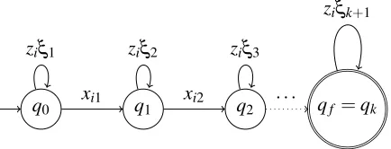
Now we describe the construction of a substitution NFAAthat substitutes, on its transition edges, new commuting/noncommuting variables for the variables (x0orx1) that it reads. LetQ={q0,q1,q2, . . . ,qk} be the states of automatonAandq0be the initial state andqk=qf be the final state.
We use the indicesi1, . . . ,ikfromLemma 2.11to define the transition ofA. The set of indices partition
each monomialmintok+1 blocks as follows.
m[1,i1−1]m[i1]m[i1+1,i2−1]m[i2]· · · ·m[ik]m[ik+1,D],
wherem[i]denotes the variable in i-th position ofmandm[i,j]denotes the submonomial ofmfrom positionsito j.
We define two new sets of variables. Theblock variablesare a set ofk+1 commuting variables
{ξ1,ξ2, . . . ,ξk+1}. There are 2kmany commutingindex variablesSj∈[k]{y0,j,y1,j}.
Now we describe the transitions of the substitution NFAA. WhileAis reading input variables in block j, it replaces eachxb,b∈ {0,1}read by the block variableξj. Itnondeterministicallydecides if
block jis over and the variable seen in the current position is an index in the isolating set. If so, A replaces the input variablexbby the index variableyb,j, and it increments the block number to j+1. Now
Awill make its transitions in the(j+1)st block as described above. The substitution map forAis given below.
For 0≤i≤k−1 andb∈ {0,1}:
δ(qi,xb) = {(qi,ξi+1),(qi+1,yb,i+1)},
δ(qk,xb) = {(qk,ξk+1)}.
Figure 1 depicts the automaton. The substitution NFA Ais described by two (k+1)×(k+1)
q0 q1 q2 qf
yb,1 yb,2 · · ·
ξ1 ξ2 ξ3 ξk+1
Figure 2: Transition diagram for the variablexbforb∈ {0,1}
More precisely, for variablexb, we take the adjacency matrixMxb of the labeled directed graph in
Figure 2, extracted from the automaton inFigure 1.
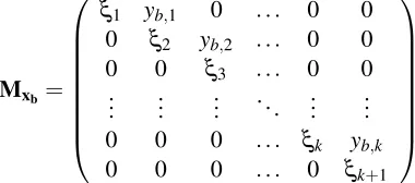
The corresponding matrixMxb of dimension(k+1)×(k+1), we substitute forxbis the following.
Mxb=
ξ1 yb,1 0 . . . 0 0 0 ξ2 yb,2 . . . 0 0 0 0 ξ3 . . . 0 0
..
. ... ... . .. ... ... 0 0 0 . . . ξk yb,k
0 0 0 . . . 0 ξk+1
The rows and the columns of the matricesMxb,b∈ {0,1}are indexed by the states of the automaton
and the entries are either block variables or index variables as indicated in the transition diagram. Let
f(x0,x1) =
t
∑
i=1ciwi.
Recall that f(x0,x1) is a polynomial with sparsity t, degree D and wi represents a monomial with coefficientcifori∈[t]. Define the matrix productwi(Mx0,Mx1)obtained by substituting the matrixMxb
forxb, b∈ {0,1}in the monomialwi, and multiplying these matrices. The following proposition is
immediate as f is a linear combination of thewi.
Proposition 4.4. Mf = f(Mx0,Mx1) =∑ t
i=1ciwi(Mx0,Mx1).
Now we are ready to proveTheorem 2.1.
Proof ofTheorem 2.1. ByProposition 2.9, we can assume that the input polynomial (given by black-box)
is a bivariate polynomial f(x0,x1)over noncommuting variablesx0andx1of sparsityt. LetM6=/0 denote the set of nonzero monomials of degreeDoccurring in f, whereD=deg(f). Then we can write the polynomial f=∑tj=1cjwjin two parts
f =
∑
wj∈M
cjwj+
∑
wj6∈M
cjwj,
Let us assume, without loss of generality, that w1 is in M and it is the monomial isolated in
Lemma 2.11. Let the isolating index set beI={i1,i2, . . . ,ik}, which means that for allwj∈M,wj|I6=w1|I
(i. e., the projections of eachwj,∀j6=1 on index setI differs from the projection ofw1). Let
w1=xb1xb2· · ·xbD,
wherebj∈ {0,1}.
We will now analyze the polynomial computed at the(q0,qf)-th entry of the matrix f(Mx0,Mx1).
Firstly, notice from the definition of the substitution NFAAthat the only nondeterminism is in picking the index set. Therefore, an index setJ={j1,j2, . . . ,jk}nondeterministically picked byAdetermines a unique computation path for it. Letwj∈Mbe a nonzero degree-Dmonomial of f. It is transformed byA into a degree-Dcommutative monomialwj,J(which is over the block and index variables) as follows. Let
ξJ = ξ1j1−1ξ2j2−j1−1· · ·ξkD+−1jk, yj,J = ya1,1ya2,2· · ·yak,k, ai∈ {0,1},
whereai=bif ji-th variable ofwjisxb. Then we have the following claim from the construction ofA.
Claim 4.5. For the index set J={j1,j2, . . . ,jk}nondeterministically chosen by the substitution NFAA,
the monomial output byAon input wj is
wj,J=ξJ·yj,J.
Notice that for two distinct index setsJandJ0we clearly have
ξJ6=ξJ0.
To see this, let j`be the first index whereJandJ0are different. Then the power ofξ`will be different in
ξJandξJ0. We thus have:
Claim 4.6. For any two index sets J,J0 and any monomial wj ∈M, the corresponding commutative monomials wj,J and wj,J0 are distinct.
We also note that the degree-kmonomialyj,J essentially encodes the projection of the degree-D
monomialwj to thekindices inJ={j1,j2, . . . ,jk}. If variablexboccurs in position jiof monomialwj it
is encoded as variableyb,iin monomialyj,J.
Claim 4.7. For each wj∈Mwe note that the(q0,qf)-th entry of the matrix wj(Mx0,Mx1)is the sum
∑
Jwj,J=
∑
JξJyj,J
over all nondeterministically picked size-k index sets J⊂[D].
To see the above claim we note that each computation path of the NFAAis determined by an index setJ along which the monomialξJyj,J is output byA. The matrix productwj(Mx0,Mx1)sums up the
Now, let fJ be the polynomial
fJ = t
∑
j=1cjwj,J=
∑
wj∈Mcjwj,J+
∑
wj∈/Mcjwj,J.
Claim 4.8. After the matrix substitution x0=Mx0 and x1=Mx1 in the polynomial f we note that the (q0,qf)-th entry of the matrix f(Mx0,Mx1)is∑JfJ.
To see the above claim we need to change the order of summation in computing the(q0,qf)-th entry
of the matrix f(Mx0,Mx1). Notice that for a fixed index setJguessed by the NFAA, for each monomial wj the NFA outputswj,J. Hence, by linearity, fixing the guessed index setJ, the NFA computes fJ on
input f. Summing over all guessed index setsJ, it follows that(q0,qf)-th entry of the matrix f(Mx0,Mx1)
is∑J fJ.
Finally, we focus on the monomialw1,Ioccurring in the polynomial∑J fJ, wherew1is the isolated monomial andIis the isolated index set.
Claim 4.9. The coefficient of w1,I in the polynomial∑J fJ is c1. As a consequence, the(q0,qf)entry of
the matrix Mf = f(Mx0,Mx1)which computes∑J fJ is nonzero.
To see the above claim we note the following:
1. For a nonzero monomialwj∈/Mof f, for each index setJof sizekthe contribution to the(q0,qf)
-th entry of -the matrix f(Mx0,Mx1)is a monomial of degree deg(wj), and deg(wj)<D. Hence,
these monomials have no influence on the coefficient ofw1,I in the polynomial∑J fJ.
2. Consider monomialswj∈M. Notice thatw1,I=ξIy1,Iand for j6=1wj,I=ξIyj,I. Now,
y1,I6=yj,I,for allwj∈M\ {w1},
becauseIis an isolating index set forMand the monomialw1is isolated. Therefore,w1,I6=wj,I
for allwj∈M\ {w1}.
It follows that the monomialswj∈M\ {w1}also have no influence on the coefficient ofw1,I in the
polynomial∑J fJ.
Hence, we conclude that the(q0,qf)-th entry of the matrixMf =f(Mx0,Mx1)is a nonzero polynomial
∑J fJ in the commuting variablesSj∈[k+1]{ξj}andSj∈[k]{y0,j,y1,j}. Moreover, the degree of polynomial ∑J fJ isD. By thePolynomial Identity Lemma 3.3it follows that the polynomial∑J fJ is nonzero in a
suitable extension of size more than(n+2)dof the fieldF.
Since the polynomial f is nonzero over the algebraMk+1(F), it is also nonzero over the algebra Mlogt+1(F). This completes the proof ofTheorem 2.1.
5
A deterministic PIT for regular circuits
Definition 5.1. A noncommutative circuitC, computing a polynomial inFhXiwhereX={x1,x2, . . . ,xn},
is+-regularif it satisfy the following properties:
• The circuit is homogeneous. The gates are of unbounded fanin.
• The+gates in the circuit are partitioned into layers (termed+-layers) such that ifg1andg2are+
gates in a+-layer then there is no directed path in the circuit betweeng1andg2.
• All gates in a+-layer are of the same syntactic degree.
• The output gate is a+gate.
• Every input-to-output path in the circuit goes through a gate in each+-layer.
• Additionally, we allow scalar edge labels in the circuit. For example, supposegis a+gate inC
whose inputs are gatesg1,g2, . . . ,gt such thatβi∈Flabels edge(gi,g),i∈[t]. If polynomialPi is
computed at gategi,i∈[t], thengcomputes the polynomial∑ti=1βiPi.
Remark 5.2. We draw the reader’s attention to the crucial fifth condition inDefinition 5.1. An important consequence of the condition is that each+-layer (other than the output and input) is a separating set for the underlying DAG of the circuitC. This property allows us to do a deterministic depth reduction of such circuits, preserving polynomial identity.
We list below some observations about+-regular circuits, and also introduce some notation in the process.
1. In a+-regular circuit, for any+gategof degree more than 1, we can assume that all inputs tog
are×-gates. This can be effected with a simple transformation to the circuit without increasing its size.
2. The+-depthof a+-regular circuitCis the number of+-layers in it. Letdbe the+-depth ofC. We number the+-layers ofCfrom bottom upward. For 1≤i≤d, letL+i denote the set of+gates in thei-th+-layer, and letL×i denote the set of×-gates which are inputs to gates inL+i . Notice that all gates inL×i andL+i have the same syntactic degreeDi. The degree of the circuitCisDd.
3. Continuing from above, we can assume that all+gates of degreeDiin the circuit are in layerL+i . Similarly, all×-gates of degreeDiin the circuit are inL×i .
4. It is clear from the structure of circuitCthat the part ofC between+-layersL+i andL+i+1 is a multiplicative circuit whose inputs are the gates in layerL+i and outputs are the gates in layerL×i+1, 1≤i≤d−1. We note that this property follows from the fifth condition inDefinition 5.1.
5. Finally, consider the bottommost+-layerL+1. We assume without loss of generality thatL×1 are the input variables, and the gates inL+1 compute homogeneous linear forms. We can ensure this by adding a dummy+-layer as the first layer 1.
In our study of+-regular circuits, it is important to consider certain special+-regular circuits of
+-depth 2. We term these as homogeneousΣΠ∗Σcircuits (as already mentioned inSection 2), in analogy
with the usualΣΠΣarithmetic circuits (see, e. g., [25]).
Definition 5.4. ΣΠ∗Σcircuit are special+-regular circuits of+-depth 2 defined as follows:
• The output gate is a+gate (which constitutes the second+-layer).
• All inputs to the output gate are×gates of the same syntactic degree.
• The gates in the first+-layer compute homogeneous linear forms (taking as input the circuit inputs).
We will require the following definition of multiplicative circuits.
Definition 5.5(Multiplicative Circuit). Let Γ={y1,y2, . . . ,yn}be a finite alphabet. Amultiplicative
circuitover the free monoid(Γ∗, .)is a directed acyclic graph with each indegree zero nodes labeled by
letters fromΓ(the inputs to the circuit). Internal nodes are concatenation gates of fanin two: its two
inputs are designated left and right child, and the gate concatenates the output of the left child with the output of the right child. A gate of the circuit is designated theoutputgate.
Remark 5.6.
• Multiplicative circuits computing words as described above are also known as a compressed context-free grammars, see, e. g., [16].
• If we letΓbe the set{y1,y2, . . . ,yn}of noncommuting variables, then a multiplicative circuit can be seen as a special kind of noncommutative arithmetic circuit that computes a single monomial in this variable set. The internal concatenation gates of the circuit are×gates.
• We sometimes allow a multiplicative circuitCto have multiple output gates. Thus, at each output gate g, the outputCg(y1,y2, . . . ,yn) computed byC is a monomial (i. e., a word) in variables
y1,y2, . . . ,yn.
• We can defineΠ∗Σcircuit as multiplicative circuits with homogeneous linear forms as input. More
precisely, letC(y1,y2, . . . ,yn)be a multiplicative circuit with output gateg, andL1,L2, . . . ,Lnbe
homogeneous linear forms in noncommuting variablesx1,x2, . . . ,xn. ThenCg(L1,L2, . . . ,Ln)is a
Π∗Σcircuit.
The following theorem is crucial to our PIT algorithm for +-regular circuits. It will allow us to decompose+-regular circuits of+-depthd into+-regular circuits of smaller+-depth, preserving homogeneous polynomial identities.
Theorem 5.7. Let T(z1,z2, . . . ,zs) be a noncommutative homogeneous degree-d polynomial over a
fieldFin noncommuting variables z1,z2, . . . ,zs. Let R1,R2, . . . ,Rs be noncommutative homogeneous
degree d0polynomials in variables x1,x2, . . . ,xnoverFsuch that{R1,R2, . . . ,Rk}are a maximal linearly independent subset of{R1,R2, . . . ,Rs}overF, where
Rj=
k
∑
i=1For fresh noncommuting variables y1,y2, . . . ,yk define linear forms
`j= k
∑
i=1αjiyi, k+1≤j≤s.
Then T(R1,R2, . . . ,Rs)≡0if and only if T(y1,y2, . . . ,yk, `k+1, . . . , `s)≡0.
Proof. The reverse implication is immediate. For, supposeT(y1,y2, . . . ,yk, `k+1, . . . , `s)≡0. Then, by substitutingRiforyi,1≤i≤kwe obtainT(R1,R2, . . . ,Rs)≡0.
We now show the forward implication. SupposeT(R1,R2, . . . ,Rs)≡0. AsR1,R2, . . . ,Rk are linearly
independent overFwe can find degree-d0monomialsm1,m2, . . . ,mk such that thek×kmatrixBof their coefficients is of full rank. More precisely, ifβjiis the coefficient ofmiinRjthen the matrix
B= (βji)1≤j,i≤k
is full rank.
Define polynomials
R0j= k
∑
i=1βjimi,1≤ j≤k, (5.1)
R0j= k
∑
i=1αjiR0i,k+1≤ j≤s. (5.2)
Notice thatT(R1,R2, . . . ,Rs)≡0 impliesT(R10,R02, . . . ,R0s)≡0. This is because every nonzero mono-mial occurring inT(R01,R02, . . . ,R0s)precisely consists of all monomials from the set{m1,m2, . . . ,mk}d
occurring inT(R1,R2, . . . ,Rs)(with the same coefficient).
Replacingmiby variableyi,1≤i≤ktransforms eachR0j to linear forms
`0j= k
∑
i=1βjiyi, for 1≤ j≤k,
and
`0j= k
∑
i=1αji k
∑
q=1βiqyq, fork+1≤ j≤s.
Note that the coefficient of any monomialyi1yi2. . .yid inT(`
0
1, `
0
2, . . . , `
0
k, `
0
k+1, . . . , `
0
s)is the same as
the coefficient of the corresponding monomialmi1mi2. . .mid inT(R01,R02, . . . ,R0s)which is zero. Hence
T(`01, `02, . . . , `0k, `0k+1, . . . , `0s)≡0. Now, sinceBis invertible, we can apply the linear mapB−1to each
Outline of the algorithm
In the following lemma we will applyTheorem 5.7to decompose+-regular circuits. Using this we will be able to design a deterministic polynomial-time PIT algorithm for+-regular circuits.
Lemma 5.8. Suppose C is a+-regular circuit of size s, syntactic degree D, and+-depth d, computing a polynomial inFhXi. For i∈[d], letL×2 ={g1,g2, . . . ,gm}. Suppose, P1,P2, . . . ,Pmare the polynomials computed at the gates g1,g2, . . . ,gm, respectively. Assume, without loss of generality, that{P1,P2. . . ,Pt} is a maximalF-linearly independent subset of{P1,P2, . . . ,Pm}, and
Pj=
t
∑
i=1αjiPi, t+1≤j≤m.
Let C0be the circuit obtained from C as follows:
(i) Delete all gates belowL×2.
(ii) Replace g1,g2, . . . ,gmby input variables y1,y2, . . . ,ym, respectively.
Then C0(y1,y2, . . . ,ym) is a +-regular circuit of +-depth d−1 and size at most s, computing a
homogeneous polynomial in y1,y2, . . . ,ym. Let C00be the circuit obtained from C0by replacing yj by the
linear form∑ti=1αjiyi, for each t+1≤ j≤m. Then the circuit C is identically zero if and only if the
circuit C00is identically zero.
Proof. The proof is an easy consequence of Theorem 5.7. LetP(x1,x2, . . . ,xn)∈FhXibe the
homo-geneous degreeDpolynomial computed byC, whereX={x1,x2, . . . ,xn}. LetT(y1,y2, . . . ,ym)be the polynomial computed by the circuitC0. LetP1,P2, . . . ,Pmbe the polynomials computed by the gates g1,g2, . . . ,gm, respectively. SinceC0is also a+-regular circuit,T is homogeneous of degree,say,D0. Each
Pi is homogeneous of degreeD00=D/D0. It follows from the structure ofCthat P(x1,x2, . . . ,xn) =T(P1,P2, . . . ,Pm).
Now, applyingTheorem 5.7 to the polynomialsP,T,P1,P2, . . . ,Pm, it follows that the circuitCis
identically zero if and only if the circuit
C0(y1,y2, . . . ,yt,
t
∑
i=1αi+1iyi, . . . ,
t
∑
i=1αmiyi)≡0.
Given a sizes+-regular circuitCof+-depthd, we can applyLemma 5.8to transformCto another
+-regular circuitC0of sizesand+-depthd−1 such that
C≡0 if and only ifC0≡0.
The pseudo-code for this procedure Prune-plus-depthis given in Algorithm A. This procedure runs in polynomial time assuming that we have a deterministic polynomial-time subroutineBasisthat computes a maximumF-linearly independent subset of a set of polynomials{P1,P2, . . . ,Pm} ⊂FhXi,
{P1,P2, . . . ,Pt}is the maximum linearly independent subset computed byBasis. We will assume that the
subroutineBasiswill also compute scalarsαji∈Fsuch that
Pj=
t
∑
i=1αjiPi, t+1≤j≤m.
In the next subsection we will describe subroutineBasis, which will complete the overall algorithm.
Prune-plus-depth
Input: A+-regular circuitCof degreeD, sizes, and+-depthd.
Output: A+-regular circuitC0of+-depthd−1 and size at mostssuch thatC≡0 iffC0≡0.
1. LetL×2 ={g1,g2, . . . ,gm}andPibe the polynomial computed atgi,1≤i≤m.
2. Notice that eachPi is computed by aΠ∗Σcircuit. Using subroutine Basis we compute a
maximum linearly independent subset, say, {P1,P2, . . . ,Pt} of {Pi |1≤i≤m}, and also
compute scalarsαji∈Fsuch that:
Pj=
t
∑
i=1αjiPi, t+1≤ j≤m.
3. Construct the pruned circuitC00as follows: in circuitCremove all gates belowL×2, and replace
gibyyi,1≤i≤t. These variables are the new inputs toC0.
4. Furthermore, inC, let the 2nd +-layer gates be L+2 ={h1,h2, . . . ,hq}. These gates
com-pute linear combinations of the gates gi,1≤i≤m. We do the rewiring so that inC00 the gatesh1,h2, . . . ,hqcompute the appropriate linear combinations ofy1,y2, . . . ,yt. Notice that
h1,h2, . . . ,hqbecomes the first+-layer forC0.
5. OutputC0.
Algorithm A
5.1 Linear independence testing ofΠ∗Σcircuits
In this subsection we solve the above mentioned linear independence testing problem. Namely, given as inputΠ∗Σcircuits computing noncommutative polynomialsP1,P2, . . . ,Pm∈FhXi, we give a deterministic
We first need to analyzeΠ∗Σcircuits. Let{L1,L2, . . . ,Lt}be the set of homogeneous linear forms (in
noncommuting variablesx1,x2, . . . ,xn) defined by the bottomΣlayers of the givenΠ∗Σcircuits computing polynomialsPi,1≤i≤m.
Without loss of generality, let{L1,L2, . . . ,Lr}be a maximal subset of{L1,L2, . . . ,Lt}such thatLi
andLj are not scalar multiples of each other for 1≤i< j≤r. Thus, for eachLi,i>rthere is some Lj,j≤rsuch thatLiis a scalar multiple ofLj. Therefore, we can express eachPi as a product of linear
forms fromL1, . . . ,Lr, upto a scalar multiple:
Pi=αiLi1Li2. . .LiD, 1≤i≤m,∀u : Liu∈ {L1, . . . ,Lr},αi∈F.
Thus, each of these polynomialsPiis, upto a scalar multiple, a product ofDmany linear forms from
the set{L1,L2, . . . ,Lr}.
Proposition 5.9. Suppose polynomials Piand Pj factorize as
Pi = αiLi1Li2. . .LiD, Pj = αjLj1Lj2. . .LjD,
where∀u : Liu,Lju∈ {L1, . . . ,Lt}. Then, Piand Pj are scalar multiples of each other iff Lju=Liu,1≤
u≤D.
Proof. The polynomialPi andPjare homogeneous degreeDpolynomials in the free noncommutative
ringFhXi. Now, it turns out thathomogeneous polynomials inFhXihave unique factorization (see,
e. g., [5, Theorem 3.4]). Furthermore, the irreducible factors are all homogeneous and their order is also uniquely determined (only scalar multiples can vary). The proposition immediately follows from this observation.
In order to analyzeΠ∗Σcircuits further, it is useful to think of aΠ∗Σcircuit computing a product
of linear forms from{L1,L2, . . . ,Lr}as a multiplicative circuit over the letters{L1,L2, . . . ,Lr}. More
formally, corresponding to the linear formsL1,L2, . . . ,Lrwe define an alphabetΓ={a1,a2, . . . ,ar}ofr letters, whereaistands forLi,1≤i≤r.
Clearly, a multiplicative circuit over(Γ∗, .)computes a word inΓ∗. Conversely, given a wordw∈Γ∗
we could ask for its compression as a multiplicative circuitCw. Such word compressions are well-studied in the literature and are closely related to the Lempel–Ziv text compression [16,21,17]. Some basic algorithmic results in this area turn out to be useful for our algorithm. We formally state these below.
Theorem 5.10(Lohrey, Plandowski, Mehlhorn et al.). LetΓ={a1,a2, . . . ,ar}be a finite alphabet.
• There is a deterministic polynomial-time algorithm that takes as input two multiplicative circuits
Ciand CjoverΓand tests if the words computed by them are identical. If not the algorithm returns
the leftmost index k where the two words differ.
• Given a word w by a multiplicative circuit C as input overΓ, the following tasks can be done in
deterministic polynomial time:
(ii) given as input an index k in binary computing the k-th letter w[k].
(iii) Multiplicative circuit Ck,k0 for the subword w[k. . .k0]for indices k and k0given in binary. In particular, it follows that the circuit Ck,k0 is of size polynomial in the sizes of C,k and k0. The
parameters k,k0are given in binary.
Remark 5.11. For 1≤i≤m, we transform theΠ∗Σcircuit computingPiinto a multiplicative circuitCi
computing a wordwiof lengthDin{a1,a2, . . . ,ar}Das follows: replace linear formLj in theΠ∗Σcircuit
by letterakifLj is a scalar multiple ofLk, fork∈[r]. Clearly,Cihas the same number of multiplication
gates as theΠ∗Σcircuit forPi.
The following lemma is immediate.
Lemma 5.12.
• The polynomials Piand Pjare scalar multiples of each other if and only if the multiplicative circuits
Ciand Cj compute the same word over{a1,a2, . . . ,ar}(i. e., iff wi=wj).
• Thus, given as inputΠ∗Σcircuits computing polynomials Piand Pj, we can check if Piand Pjare
scalar multiples of each other in deterministic polynomial time.
Proof. The first part of the lemma follows directly from Proposition 5.9. The second part follows
immediately fromTheorem 5.10.
Our aim is to efficiently determine a maximal linearly independent subsetAofP1,P2, . . . ,Pr, and
express eachPi6∈Aas a linear combination of polynomials inA. The difficulty is that thePi, which are
given byΠ∗Σcircuits of sizes, can have degree exponential ins.
Our approach, that circumvents this difficulty, will crucially require a rank bound due to Saxena and Seshadhri [25] obtained in their study ofcommutativeΣΠΣarithmetic circuits. We recall the Saxena–
Seshadhri result. Consider aΣΠΣarithmetic circuitC0, where the topΣgate has fanink, allΠgates are of
faninD, and eachΠgate computes a productQi,1≤i≤kof homogeneousF-linear forms incommuting
variablesy1,y2, . . . ,yn. CircuitC0is said to besimpleif the gcd(Q1,Q2, . . . ,Qk) =1. CircuitC0is said to
beminimalif for any proper subsetS⊂[k]the sum∑i∈SQi6=0.
Theorem 5.13(Saxena, Seshadhri). Let C0be a simple and minimalΣΠΣarithmetic circuit of the form
C0(y1,y2, . . . ,yn) = k
∑
i=1D
∏
j=1Li j,
where Li jare homogeneous linear forms in commuting variables y1,y2, . . . ,yn. If the polynomial computed
by C0is identically zero then the rank of the set{Li j|1≤i≤k,1≤j≤D}of allF-linear forms occurring
at the bottomΣlayer of the circuit is bounded by O(k2logD).
This line of research, analyzing the rank of linear forms occurring inΣΠΣidentities, was initiated by
Noncommutative to commutative
For applying the rank bound ofTheorem 5.13, we make the polynomialsPi,1≤i≤`commutative and
set-multilinear in variables{xim|1≤i≤n,1≤m≤D}as follows:
For each linear formLj=∑ni=1γjixi,1≤j≤rdefineDmany linear forms:
L0jm= n
∑
i=1γjixim,1≤m≤D,
wherexim, for 1≤i≤nand 1≤m≤Dare new distinctcommutingvariables. Define polynomials ˆPi
fromPi as
ˆ
Pi= D
∏
m=1L00im,
whereL00im=L0jm ifLim=Lj,j∈[r]. In other words, we obtain the set-multilinear polynomial ˆPifromPi
by replacing them-th linear form, sayLj, withL0jm, for 1≤m≤D.3
The following observation follows easily from the above definition of the polynomials ˆPi.
Lemma 5.14. Consider the set-multilinear polynomialsPˆi,1≤i≤m defined above. A linear form L0
divides the gcd of{Pˆi|i∈S}for a subset S⊆[m]if and only if L0=L0jmfor some j∈[r]and m∈[D],
and the linear form Lj occurs in the m-th position of each Pi,i∈S.
Proof. IfL0divides gcd of{Pˆi|i∈S}, it follows thatL0=L00imfor somem∈[D]for eachi. But giveni, L00im=L0jmfor some j∈[r]. It follows thatLjmust occur atm-th position in each of the noncommutative
productsPi. The reverse implication is also immediate.
The next lemma explains the importance ofTheorem 5.13to the problem of computing a maximum independent subset of{Pi|i∈[m]}.
Lemma 5.15. Suppose the polynomial Pican be expressed as anF-linear combination of the polynomials P1,P2, . . . ,Pi−1. Let
S={j∈[i−1]|deg(gcd(Pˆi,Pj))ˆ ≥D−c·m4},
where c>0is some absolute constant. Then Pican be expressed as a linear combination of polynomials
from the subset{Pj|j∈S}.
Proof. Suppose Pi is expressible as an F-linear combination of P1,P2, . . . ,Pi−1. Let S⊆[i−1] be a
minimal subset such that we can write
Pi=
∑
j∈S
γjPj, γj6=0 for all j.
Now, consider the set-multilinear circuitC0defined by the sum of products ˆ
Pi−
∑
j∈S
γjPjˆ .
By minimality of subsetS, circuitC0 is minimal. Suppose for some j∈S, Pi and Pj disagree onρ
positions, whereρ> `4. That is, for more than`4 positionsm, the linear forms occurring in them-th position inPiandPjare different. Let the gcd of the polynomials in the set{Pjˆ | j∈S} ∪ {Pˆi}beP, and
let deg(P) =δ. ByLemma 5.14it follows that
δ ≤D−ρ.
Define polynomialsQi=Pˆi/PandQj=Pjˆ/P,j∈S. Notice that eachQi is a product ofD−δ linear
forms. Furthermore,
ˆ
Pi−
∑
j∈S
γjPˆj=P(Qi−
∑
j∈SγjQj).
Consider the simple and minimal circuitC00defined by the sum
Qi−
∑
j∈S
γjQj.
Clearly,C0 is zero iffC00is zero. SinceC00is aset-multilinearcircuit, the rank of the set of allF-linear
forms is at leastD−δ (as linear formsL0jmandL0j0m0 form6=m0have disjoint support). Now, ifC00≡0 then by the Saxena-Seshadhri rank bound [25] we haveρ≤D−δ≤O(`2log(D−δ)). Hence, it follows
from the inequality log2x≤x1/2thatρ≤c·`4, for some constantc>0. Thus, for each j∈S,P
i andPj
can disagree on at mostc·`4positions. This proves the lemma.
UsingTheorem 5.10we can efficiently determine ifPiandPjgiven byΠ∗Σcircuits disagree on at
most, say,qpositions,qgiven in unary.
Lemma 5.16. Let Piand Pj be noncommutative homogeneous degree-D polynomials inFhXi, given as
Π∗Σcircuits of size at most s, where the first+-layer computes homogeneous linear forms L1,L2, . . . ,Lr
which are not scalar multiples of each other. Then in deterministic time polynomial in s,n,q we can
determine if Pi and Pj differ in at most q positions, and if so, we can also determine those positions and
the linear forms at those positions.
Proof. The proof is a simple application ofTheorem 5.10. First, as explained inRemark 5.11we obtain
sizesmultiplicative circuitsCi andCj over lettersai corresponding to the linear formsLi,1≤i≤r. Letwi andwj be the lengthDwords computed byCi andCj respectively. Applying the algorithm of Theorem 5.10we can check ifCiandCj compute identical words or find the leftmost indexksuch that
wi[k]6=wj[k]. ByTheorem 5.10we can compute circuitsCi0andC0j for the suffixeswi[k+1· · ·D]and
wj[k+1· · ·D]ofwiandwj starting at(k+1)-th position, and again look for the leftmost index where
they differ. We need to run this iteration at mostq+1 times to determine allqpositions wherePiandPj
differ, and if so, also find the linear forms at those locations.
Before we design the algorithm for finding a maximum independent subset of{Pi|i∈[m]}, we need
Lemma 5.17. Let P0, P10,P20, . . . ,Ps0 be homogeneous degree-d noncommutative polynomials in FhXi,
each given by an ABP as input. Then, in deterministic polynomial time we can determine if P0can be
expressed as anF-linear combination of the Pi0,1≤i≤s, and if so, we can compute scalarsαi∈Fsuch
that
P0=
s
∑
i=1αiPi0.
Proof. Let B be the input ABP forP0, and Bi be the given ABP forPi0,1≤i≤s, respectively. Let
X={x1,x2, . . . ,xn}.
For each monomialm∈Xd, letvm∈Fsdenote the vector of the coefficients ofmin the polynomials Pi0,1≤i≤s. More precisely,vm[i]is the coefficient ofminPi0,1≤i≤s. Letcmdenote the coefficient of min the polynomialP0. Then we observe that
P0=
s
∑
i=1αiPi0
if and only if for all monomialsm∈Xd
cm=
s
∑
i=1vm[i]·αi. (5.3)
Equation (5.3)cannot direct give an efficient algorithm as there arend many equations to contend with. However, we will show, exploiting the fact that thePi0 are given as input by ABPs, that we can efficiently reduce the number of equations to polynomially many, which can then be efficient solved for theαi.
Let y and z be two fresh noncommuting variables. Consider the noncommutative polynomial ˆ
P=∑si=1yPi0z. It is homogeneous of degreed+2 and is computed by an ABP ˆBobtained by combining
the ABPsBi,1≤i≤swith a new start node and sink node as follows:
• Create a new start nodes0and introduce directed edges froms0to the start node ofBilabeled by
variableyfor 1≤i≤s.
• Create a new sink nodet0and introduce directed edges from the sink node ofBitot0labeled by variablezfor 1≤i≤s.
Clearly, ˆBcomputes the polynomial ˆP.
Based on Raz and Shpilka’s work [23], we now define aRaz-Shpilka basisfor layeriof the ABP ˆ
P. Let the number of nodes at layeribeni and let{p1,p2, . . . ,pni} be the polynomials computed at the nodes. Consider theni×nimatrixLiwhose rows are indexed by degree-imonomials, and the j-th
column, 1≤j≤ni, is the coefficient vector ofpj. ARaz-Shpilka basisfor layeriis a set of at mostni
degree-imonomials such that the corresponding rows ofLiis a basis for the row space ofLi. Notice that every degree-imonomial is identified with a row vector ofLi. Following Raz and Shpilka [23], as also
elaborated subsequently [6, Theorem 3.4], we can compute a Raz-Shpilka basis for every layer of the given ABP ˆPin deterministic polynomial time. In particular, consider a Raz-Shpilka basisMfor the
the ABPsB1,B2, . . . ,Bs. Thus,Mis a collection of at mostsmonomials. Without loss of generality, we
can assume thatM={ym1,ym2, . . . ,yms}, wheremi∈Xd,1≤i≤s.
SinceMis a Raz-Shpilka basis, it follows that for any monomialm∈Xdthe coefficient vectorvm
is in the linear span of{vmi |1≤i≤s}. Next, we can compute the coefficient cmi of monomial mi
in the polynomialP0 (from the input ABPB) in deterministic polynomial time [23,6]. It follows that
α1,α2, . . . ,αssatisfiesEquation (5.3)if and only if it satisfies the followingslinear equations:
cmj=
s
∑
i=1vmj[i]·αi,1≤ j≤s. (5.4)
Now, using Gaussian elimination, in polynomial time we can check feasibility ofEquation (5.4)and compute a solution.
We are now ready to prove the result of this subsection.
Theorem 5.18. Given as inputΠ∗Σcircuits computing noncommutative polynomials P1,P2, . . . ,Pm∈
FhXi, there is a deterministic polynomial-time algorithm that will find a maximal linearly independent
subset A of the polynomials Pi,1≤i≤m, and also express the others asF-linear combinations of the Pi
in A.
Proof. The algorithm for computing a maximal linearly independent subsetAofP1,P2, . . . ,Pmworks as
follows: IncludeP1inA. Fori≥2, includePi inAiff it is linearly independent of{P1,P2, . . . ,Pi−1}. Thus, the problem boils down to checking ifPiis linearly independent ofP1,P2, . . . ,Pi−1. Following
Lemma 5.15let
S={j∈[i−1]|deg(gcd(Pˆi,Pˆj))≥D−c·m4},
whereDis the degree of each of the polynomialsPi,1≤i≤mandc>0 is some absolute constant. By Lemma 5.15it suffices to check ifPiis linearly independent of{Pj| j∈[i−1]such that j∈S}.
ByLemma 5.16we can efficiently compute the subsetS, and the subsetI ⊂[D]of at mostc·m5
many positions such thatPi agrees with everyPj,j∈Sin all positions in[D]\I. DefinePi0=∏u∈ILiu
andP0j=∏u∈ILjufor all j∈S. The following claim is immediate. It follows from the fact that for every
positionu∈[D]\I the linear formsLiu andLju,j∈Sare all identical.
Claim 5.19. Pi is linearly independent of {Pj | j∈S} if and only if Pi0 is linearly independent of
{Pj0| j∈S}.
Thus it suffices to check ifPi0is linearly independent of{P0j| j∈S}. Each of these polynomials is a product of at mostcm5many linear forms. Since a product of linear forms can clearly be seen as an ABP, we can apply the algorithm described inLemma 5.17to check this in polynomial time.
To conclude the overall proof we note that Algorithm B below can be applied to determine the leftmost maximal linearly independent subsetAof the input polynomialsP1, . . . ,Pmand also express the
Linear-Span
Input:Π∗Σcircuits for polynomialsP1,P2, . . . ,Pi.
Output: Check whetherPican be expressed as a linear combination of{P1,P2. . . ,Pi−1}or not. If so, find such an expression.
1. LetLi,i∈[r]be the linear forms computed at the bottom+-layer of the input circuits such that they are not multiples of each other.
2. Find corresponding multiplicative circuitsCj,j≤iover lettersai,i∈[r]corresponding to the Li. UsingLemma 5.16, determineS⊆[i−1]such thatCiandCjdiffer in at mostcm4positions
and find the letters occurring in those positions.
3. LetI ⊂[D]be the set of at mostcm5 positions wherePi differs from somePj,j∈S, and
compute the polynomialsPi0andP0j,j∈Sby dropping the linear forms occurring in all other positions.
4. UsingLemma 5.17determine ifPi0is can be expressed as a linear combination ofP0j,j∈S. If so, then the same linear expression will hold forPiandPj,j∈Sand is the output.
Algorithm B
Finally, we describe Algorithm C, which is the basis finding algorithm.
Basis
Input:Π∗Σcircuits for polynomialsP1,P2, . . . ,Pm.
Output: A maximumF-linearly independent subsetAof{P1,P2, . . . ,Pm}.
1. A:={P1}.
2. Fori=2 tomdo: IfPiis linearly independent of{P1,P2, . . . ,Pi−1}thenA:=A∪ {Pi}. (This
is tested using Algorithm B).
3. OutputA.
The main result of this section is now a simple consequence ofLemma 5.8.
Proof ofTheorem 2.5. Let the input+-regular circuitCbe of sizesand+-depthd. ByLemma 5.8, using
Algorithm A we can transform, in deterministic polynomial time,Cinto a+-regular circuitC0of size bounded bysand+-depthd−1 such thatC≡0 if and only ifC0≡0.
On repeated application we finally obtain aΣΠ∗Σcircuit ˆCof size at mosts, for which we need to do polynomial identity testing. The polynomial ˆPcomputed by ˆCis of the form
ˆ
P=
m
∑
i=1αiPi, (5.5)
where eachPiis computed by aΠ∗Σcircuit of size at mosts, andPm=∏Dj=1Ljm, where eachLjmis from
the set of linear forms{L1,L2, . . . ,Lt},t≤soccurring at the bottom+-layer of circuitC.
We can now applyTheorem 5.18to find a maximal linearly independent subset{Pj| j∈S},S⊆[m]
of{P1,P2, . . . ,Pm}, and express eachPi,i6∈Sas a linear combination of polynomials in {Pj | j∈S}.
Substituting these expressions inEquation (5.5)and collecting coefficients we will obtain
ˆ
P=
∑
j∈S
βjPj,
which, by linear independence of{Pj|j∈S}is identically zero iff eachβj is zero.
6
Black-box randomized PIT for homogeneous
ΣΠ
∗Σ
In this section we give a randomized black-box PIT algorithm forΣΠ∗Σcircuits.
ByTheorem 2.5we can test if a given homogeneousΣΠ∗Σcircuit (white-box) is identically zero in
deterministic polynomial time. However, suppose we have only black-box access to aΣΠ∗ΣcircuitC
computing a polynomial inFhXi. In other words, we can evaluateCon square matricesMi substituted
forxi,1≤i≤n, where the cost of an evaluation is the dimension of theMi. The results inSection 5
exploit the input circuitC, and hence are not applicable. Specifically,Cmay compute an exponential degree noncommutative polynomial, but it is not clear if we can test whetherC≡0 by evaluating it on polynomial dimension matrices. Neither is the black-box PIT ofSection 4applicable, sinceΣΠ∗Σcircuits
can compute polynomials with a double-exponential number of monomials.
SupposeCis ans-sumP1+P2+· · ·+PsofD-products of linear forms in variablesX. That is,
Pi=Li1Li2. . .LiD,
whereDis exponential. Then we show thatC6≡0 iffCis nonzero on randomO(s)×O(s)matrices with entries fromFor a suitably large extension ofF. The proof is based on the notion of projected
6.1 Projected polynomials
Definition 6.1. Let P∈FhXibe a homogeneous degree-Dpolynomial. For an index setI⊆[D]the
I-projectionof polynomialPis the polynomialPIwhich is defined by letting all variables occurring in
positions indexed by the setI as noncommuting. In all other positions we make the variables commuting, by replacingxiwith a corresponding commuting variablezifor 1≤i≤n. Thus, theI-projected polynomial
PI is inF[Z]hXi, and the (noncommutative) degree ofPI, which is its degree only in theX variables, is|I|.
Lemma 6.2. Let P1,P2, . . . ,Ps∈FhXieach be a product of D homogeneous linear forms
Pi=Li,1Li,2. . .Li,D,
where{Li,j: 1≤i≤s,1≤ j≤D}are linear forms inFhXi. Then, given any scalarsβ1,β2, . . . ,βs∈F
there exists a subset I⊆[D]of size at most s−1such that
s
∑
i=1βiPi=0iff s
∑
i=1βiPi,I=0,
where Pi,I∈F[Z]hXiis the I-projection of the polynomial Pi.
Proof. The proof is by induction ons. The lemma clearly holds for the base cases=1, becauseP1,/0,
which is a product of linear forms inF[Z], is nonzero iffP1is nonzero.
By induction hypothesis, we assume that an index set of size at mosts−2 exists for any set of at mosts−1 polynomials inFhXi, each of which is a product ofDhomogeneous linear forms. The forward
implication is obvious, because making variables commuting can only facilitate cancellations. We prove the reverse implication.
Suppose∑si=1βiPi 6=0 forβi∈F,1≤i≤s. Let j0∈[D]be the least index, if it exists, such that
rank{L1,j0, . . . ,Ls,j0}>1. If no such index exists then thePi are all scalar multiples of each other. Then
∑si=1βiPi=αP1, for someα∈F, which is zero if and only ifαP1,/0is zero (by the base case), proving the implication.
We can assume, by renumbering the polynomials, that{L1,j0, . . . ,Lt,j0}is a maximal linearly
inde-pendent set in{L1,j0, . . . ,Ls,j0}, wheret>1.
Then,
Pi=ciPLi,j0Li,j0+1. . .Li,D: 1≤i≤t,
Pi=ciP· t
∑
k=1γk(i)Lk,j0
Li,j0+1. . .Li,D:t+1≤i≤s,
where{ci∈F: 1≤i≤s},{γk(i)∈F: 1≤k≤t,t+1≤i≤D}, andP∈FhXiis a product of homogeneous
linear forms (or a scalar). For 1≤i≤s, let
Pi0=ci D