A constrained minimum spanning tree problem
Alberto PerettiDepartment of Economics, University of Verona Verona, Italy
e-mail: [email protected] December, 2018
Abstract
In the classical general framework of the minimum spanning tree problem for a weighted graph we consider the case in which a predetermined vertex has a certain fixed degree. In other words, given a weighted graph G, one of its vertices v0 and a positive integer k, we
consider the problem of finding the minimum spanning tree ofGin which the vertexv0has
degreek, that is the number of edges coming out ofv0.
We recall that among the various methods for the solution of the unconstrained problem an efficient way to find the minimum spanning tree is based on the simple procedure of choosing one after the other an edge of minimum weight that has not be chosen yet and does not create cycles if added to the previously chosen edges. This technique is known as the “greedy algorithm”. There are problems for which the greedy algorithm works and problems for which it does not.
We prove that for the solution of the one degree constrained minimum spanning tree problem the classical greedy algorithm finds a right solution.
Keywords. Graph theory, Trees, Minimum spanning tree problem, Constrained minimum spanning trees.
AMS Classification. 05C05, 05C85
1
Introduction
Among the combinatorial optimization problems the well known MST (Minimum Spanning Tree) problem consists in finding a spanning tree of minimum cost over a connected weighted graph. It is a classical problem for which many efficient algorithms have been proposed. The problem can be solved in polynomial time in the number of nodes of the given graph.
In the literature many variations of the original problem have been considered during the years. For example, a very general formulation can be the following: given a connected weighted graphG, find a minimum spanning tree for Gthat satisfies a property P, that is a property of trees, usually assumed to be valuable in polynomial time. The new problem may be indicated as an MST(P)problem. In [1] the case whenP is an isomorphism property is considered, that means the tree is required to be isomorphic to a certain model of trees.
Another large class of specification of the original MST problem is the Degree-constrained MST problem. Here the required tree has some constraint on the degree of its nodes. For example the constraint can be to ask for a tree in which all the nodes have degree not greater than a fixed positive integer k. This is known to be a difficult problem.
We aim here to consider a particular case in the Degree-constrained MST problem: in the graph we fix the attention on a particular node and we ask in the optimal tree this node has a predefined fixed degree.
2
Notations and problem definition
2.1 Notations
Let us introduce some of the basic vocabulary and notions of graph theory.
An undirected graph (graph for short in the following)G is a pair G= (V, E) whereV is a finite set of vertices andE is a finite set of edges, each one connecting two vertices. We may see the set E as a subset of non ordered pairs of vertices: if e∈ E, then eij = (vi, vj),vi, vj ∈V.
The two vertices are called the neighbors of the edge. The pairs are non ordered, as we are considering undirected graph.
The degree of a vertexv is the number of edges havingv as a neighbor. Equivalently, if we define the neighbors of v as the setN(v) ={w∈V : (v, w)∈E}, the degree ofv is|N(v)|.
A path p(u, v) in a graph G = (V, E) from vertex u ∈ V to vertex v ∈ V is a sequence p(u, v) = (u, v1, v2, . . . , vk, v) of vertices of V such that (u, v1),(vk, v) ∈ E, and (vi, vi+1) ∈ E for i= 1, . . . , k−1.
A path p(u, v) in G with u = v is called a cycle in G. The length |p(u, v)| of a path p(u, v) = (u, v1, v2, . . . , vk, v) is defined byk+ 1, namely the number of edges between u andv
inp(u, v).
A graph is connected if for any two vertices uand v inV there is a pathp(u, v) going from u to v. A tree is a connected graph with no cycles.
We call a forest a set of trees whose vertices are disjoint.
If G= (V, E) is a connected graph, a spanning tree for Gis a tree(V, E0)whereE0 ⊆E. We will be dealing with weighted graphs, in the sense a positive cost function is defined on the set of edges inG. We have then c:E →R+. If(u, v)∈E, the value c(u, v) is the cost of the edge(u, v).
2.2 Problem definition
Let G= (V, E) be a connected weighted graph, whereV ={v1, v2, . . . , vn} is the vertex set of
Gand E ={e1, e2, . . . , em}is the edge set of G. Letwi represent the weight or cost of edge ei,
for i= 1, . . . , m, where the weight is restricted to be a nonnegative real number.
The Minimum Spanning Tree problem consists in finding a spanning tree ofGwith minimum cost. Formally, we may describe any subgraph of G by means of a vectorx = (x1, x2, . . . , xm)
where each component xi is defined as
xi=
(
1 if edgeei is in the subgraph
0 otherwise.
Remembering that a subgraph S of G is a spanning tree of Gif S contains all the vertices ofG, is connected and contains no cycles, let’s callT the set of all the spanning trees ofG. The MST problem is the problem
minnz(x) = m X i=1 wixi : x∈T o .
Now, suppose we want to set constraints on the degree of vertices in G. Of course we may think of equality/inequality constraints. Ifbj is the constraint on the degree d(vj) of vertex vj,
then the general Degree-constrained Minimum Spanning Tree problem is the problem
min n z(x) = m X i=1 wixi : d(vj)≤bj, vj ∈V, x∈T o .
In this framework, ifkis a positive integer, we have a k-bounded MST problem ifbj =kfor
each j.
We want to consider here a simpler case of a Degree-constrained Minimum Spanning Tree problem, given by an equality constraint on one vertex ofG, let’s say v1. The problem is then
minnz(x) = m X i=1 wixi : d(v1) =k, v1 ∈V, x∈T o .
3
Elementary operations in a graph
LetG= (V, E) be a connected weighted graph and letT = (V, E0) be a spanning tree of G. Definition 1. If ais an edge belonging toe\E0 and bis an edge in the cycle created by adding
ato the tree T, we say we are doing an elementary operation onT in adding aand taking offb. Remark. By performing an elementary operation on a spanning tree of G we end up with another spanning tree ofG. We call the valuec(a)−c(b)the cost of the elementary operation. It is possible to characterize minimum spanning trees of a graph by means of elementary operations. In fact the following theorem holds.
Theorem 1. A spanning tree T of G is minimum if and only if every elementary operation on
Proof. If T is minimum then every elementary operation on T has necessarily a nonnegative cost. Let’s suppose that inT every elementary operation has a nonnegative cost and let T0 be a minimum spanning tree of G. Suppose a1, a2, . . . , as are the edges in A0 (the order is not relevant) and b1, b2, . . . , bs the ones in A. If the two sets of edges are not equal, let bk the first
edge in A that does not belong to A0. If we addbk to A0 and we take out bk from A we get a
cycle in A0: in this cycle there is an edge ah, different from bk, that does not belong to A and
reconnects Aafter the remotion of bk. Then
c(bk)−c(ah)≥0as an elementary operation on A0, which is minimum;
c(ah)−c(bk)≥0by the assumption, as an elementary operation on A.
Hence we have a null cost elementary operation onA0that gives us a new minimum spanning tree A1 with one edge more in common with A. If A and A1 are not equal, we can repeat the step more and more till we get the trees with the same set of edges and the same cost.
Let us introduce the concept of partition in a graph.
Definition 2. We call partition forest of the graph G with roots v1, . . . , vp a forest with p
con-nected components which contains all the vertices of G and such that each component contains just one of the nodes v1, . . . , vp.
Also for the partition forests we may define an elementary operation.
Definition 3. Given a partition forest F with roots v1, . . . , vp, adding an edge and removing
another edge in the cycle that has been created, in such a way we end up again with a partition forest with the same roots, is called an elementary operation on the partition forest F.
Remark. For as a partition forest with rootsv1, . . . , vp two kinds of elementary operations may
exist. The first kind corresponds to the elementary operations on a tree and consists in an operation internal to one of the connected components of the forest. The second kind consists in a connection operation of two different components and the consequent disconnection of the same components. In the same way we did for the trees, it is possible to characterize a minimum spanning forest by means of elementary operations.
Theorem 2. A partition forestF with rootsv1, . . . , vp is minimum if and only if every
elemen-tary operation on F has a nonnegative cost.
Proof. If F is minimum then every elementary operation on T has necessarily a nonnegative cost. Let’s suppose in F every elementary operation has a nonnegative cost and let F0 be a minimum partition forest with roots v1, . . . , vp.
Suppose a1, a2, . . . , as are the edges in F0 and b1, b2, . . . , bs the ones in F. If the two sets
of edges are not equal, let bk the first edge in F that does not belong to F0. Let’s add bk to
F0 and remove bk from F. In F0 either we create a cycle in one connected component or we connect two different components. InF we just create a new connected componentC that does not contain any of the roots. Now it is easy to see that either in the created cycle or in the path that connects the two roots we have an edgeah, different frombk, that reconnectsCto the rest
of the forest. Then
c(bk)−c(ah)≥0as an elementary operation on F0, which is minimum;
c(ah)−c(bk)≥0by the assumption, as an elementary operation on F.
Adding in F0 bk and removing ah is then a null cost elementary operation that gives us a
new minimum forest with one edge more in common with F. We can repeat the steps till we get the same forests.
Remark. Clearly Theorem 1 is just a particular case of Theorem 2, as a spanning tree is a partition forest with root v, wherev is any node in the graph.
4
Two algorithms to find a minimum partition forest
4.1 A first algorithm for a minimum partition forest
Here is an algorithm for the search of a minimum partition forest with roots v1, . . . , vp in a
connected weighted graph G = (V, E, c). We indicate with F = (V, E0) the forest; if |V|= n then|E0=n−p|. Algorithm 1 begin E0:=∅; while|E0| 6=n−p do begin
sia e uno spigolo minimo, e /∈ E0, che aggiunto adE0 non forma cicli e non connette due radici;
E0:=E0∪ {e}
end end
Theorem 3. Algorithm 1 finds a minimum forest with roots v1, . . . , vp.
Proof. The output of Algorithm 1 is certainly a forest with rootsv1, . . . , vp. LetF be this output
and let F0 be a minimum forest with roots v1, . . . , vp. If F and F0 have the same edges, the result is proved; otherwise let’s give these edges the same order in which they have been selected by the algorithm. If a1, . . . , as are the edges, then for everyi ai is a minimum edge that, added
to a1, . . . , ai−1, does not create cycles and does not connect two roots. Moreover let us give the edges in F0 any ordering we want: beb1, . . . , bs these edges. Let ak be the first edge in F that
does not belong to F0 and let us addak to F0. We may have two cases:
1. We get a cycle in one of the connected components inF0. In this cycle there is an edgeb that does not belong toF; consider thatb, if added toa1, . . . , ak−1, does not create cycles and does not connect two roots, as a1, . . . , ak−1 belong to F0. Then c(b) ≥c(ak). Hence
if inF0 we add ak and we removeb we get a forestF00 with cost less than or equal to the cost ofF0. As the strict inequality can not hold, beingF0 minimum, thenc(F00) =c(F0). Hence F00 is a minimum forest with roots v1, . . . , vp that has one more edge than F0 in common with F. Now, if F and F00 have the same edges, the result is proved; otherwise we can repeat the procedure.
2. Two roots vi andvj are connected inF0. In the pathvi. . . vj just created there is an edge
bthat does not belong toF; if added toa1, . . . , ak−1,bdoes not make a cycle and does not connect two roots, as a1, . . . , ak−1 belong to F0. Then c(b) ≥c(ak). The same as before,
inF0 we may add ak and removeb, getting a forest F00 with rootsv1, . . . , vp and cost less
than or equal to the cost of F0. As the equality must hold, F00 is a minimum forest with rootsv1, . . . , vp that has one more edge thanF0 in common with F. The conclusions are the same as in the first case.
Remarks. Algorithm 1 operates on a partition forest in the same way Kruskal’s algorithm operates on a spanning tree. It is a so called greedy algorithm: this is referred to the technique
of choosing at each step a minimal element that preserves the structure of the object we want to construct. It is interesting that the greedy technique works for certain types of problems and does not for others. The concept of matroid investigates on this aspect.
4.2 Another algorithm for a minimum partition forest
Here is a different algorithm for the search of a minimum partition forest with rootsv1, . . . , vp
in a connected weighted graphG= (V, E, c). We still indicate withF = (V, E0) the forest. Algorithm 2
begin
set up a minimum spanning treeT = (V, S) for G; roots:={v1};
E0:=T;
fori= 2to p do begin
letvs be the root to which vi is connected inF = (V, E0);
letebe a maximum edge in the path vi. . . vs;
E0:=E0\ {e}; roots:=roots∪ {vi}
end end
Theorem 4. Algorithm 2 finds a minimum forest with roots v1, . . . , vp.
Proof. LetF be the output of Algorithm 2: clearlyF is a partition forest with roots v1, . . . , vp.
We prove it is minimum by showing that every elementary operation on F has a nonnegative cost, using Theorem 2.
If we consider an elementary operation internal to one of the components, consisting in adding an edge a and removing an edge b in the cycle that has been created, certainly c(a) ≥c(b) as otherwise the spanning tree T obtained in the first part of the algorithm would have not been minimum. Let’s consider now an elementary operation involving two different components that consists in connecting them by adding the edge a and disconnecting them again by removing the edge b in the path that joins the two roots. If abelongs to the tree T thena is maximum in this path and c(a) ≥ c(b). If a does not belong to T, then in T the two components are connected by an edgec; obviouslyc(a)≥c(c) becauseT is minimum andc(c)≥c(b) becausec is maximum in the path that joins the two roots: also in this case thenc(a)≥c(b).
5
Minimal spanning trees with one degree constraint
LetG= (V, E, c)be again a connected weighted graph, let v0 one of its nodes and k a positive integer.1 We want to solve the following problem: find a minimum spanning tree of Gin which the degree ofv0 isk. As we said in the footnote, we assume that the degree ofv0 inGis at least
k. We assume also that we do not disconnect Gby removing any of the incident edges inv0. A spanning tree of Gwithdeg(v0) =kcan be represented as in Figure 1.
We may think of v1, . . . , vk as the roots of the tree. Everything is underneath the roots in
the picture must be intended as a subtree and will be called a component of the tree. The nodes
1For the meaningkhas in the following, we assume thatk is not greater than the degree ofv
0 in the graph
v0
v1 v2 . . . vk
Figure 1: A model for a tree with deg(v0) = k. The triangular structures below the roots have to be intended as subtrees.
of the components will be the “descendants” of their roots. These names are the same we have with the partition forests: in fact the components of the tree are nothing but a partition forest with rootsv1, . . . , vp for the subgraph ofGgenerated by the nodes other thanv0.
The following theorem can be easily proved.
Theorem 5. If(v0, v1)is a minimum cost edge among the incident edges inv0 then a minimum spanning tree forG exists with deg(v0) =k that contains(v0, v1).
Proof. LetT(k) be a minimum spanning tree of Gwith deg(v0) =k. If T(k) does not contain (v0, v1) suppose in T(k) v1 is a descendant of the root v2. If(v0, v1) was not a minimum cost edge incident inv0, the tree we obtain fromT(k) by adding(v0, v1)and removing(v0, v2)would be a tree with deg(v0) = k with cost less than T(k). This contradicts the assumption T(k) is minimum. hence (v0, v2) is a minimum cost edge incident in v0, the same as (v0, v1): the tree we obtain by adding(v0, v1)and removing(v0, v2)is then the minimum spanning tree ofGwith deg(v0) =k we were looking for.
Also for the trees with deg(v0) =k it is worthwhile to introduce the concept of elementary operation, as it will be used in the following proofs. Since we want an elementary operation not to modify the essential characteristics of the structure, for trees with deg(v0) =k we consider elementary operations preserving the degree of v0.
BeT(k) then a minimum spanning tree ofGwithdeg(v0) =k. An elementary operation on
T(k) preserving the degree ofv0 may be of three types:
1. (Root change in a component): if in T(k) v2 descends from v1, the elementary operation consists in adding the edge(v0, v2) and removing the edge(v0, v1).
2. (On the components): it is an operation that does not involve the edges incident inv0; in other words it is an elementary operation on the forest of the components ofT(k). 3. It consists in the following sequence of operations: addition of an edge(v0, v2), removal of
an edge anon incident in v0 in the generated path, removal of an edge (v0, v1) and final addition of an edgeb that reconnects the tree.
Remarks. It is evident that the result of an elementary operation preserving the degree of v0 is a tree with deg(v0) =k. In the following, talking about elementary operations on a tree with deg(v0) =k we will intend elementary operations preserving the degree of v0.
We present an algorithm for the search of a minimum spanning tree of Gwithdeg(v0) =k. Algorithm 3
begin
set up a minimum spanning treeT = (V \ {v0}, S) forGfor the subgraph ofG generated by the nodesV \ {v0};
let (v0, v1)a minimum edge incident in v0;
S :=S∪ {(v0, v1)}; roots:={v1}; while |roots| 6=kdo
begin
for each node v such that (v0, v) exists with v /∈roots, let ebe a maximum edge non incident in v0 in the pathv . . . v0;
computec0(v) =c(v0, v)−c(e); let u be a node with minimum c0(u); S :=S∪ {(v0, u)} \ {e};
roots:=roots∪ {u}; end
end
Theorem 6. If T(k) is a minimum spanning tree of G with deg(v0) = k and v1. . . vk are its
roots, then a minimum tree T(k+ 1) exists with deg(v0) =k+ 1whose roots are v1. . . vkvk+1. Proof. In order to facilitate the notations we give the proof in the case n = 4, but there is a general validity. Suppose T(4) and T(5) are minimum spanning trees with deg(v0) = 4 and deg(v0) = 5 respectively. v0 v1 v2 v3 v4 T(4) v0 v v 3 T(5)
Let’s assume that for example v3 is not a root inT(5): we want to show that we can always find a minimum T0(5)in which v3 is a root.
Let’s assume v3 is descendant of the rootv. If in T(4) v descends from v3 we can make in both trees an elementary operation of type 1:
(inT(5)): ∪{(v0, v3)} \ {(v0, v)}has nonnegative cost asT(5)is minimum, (inT(4)): ∪{(v0, v)} \ {(v0, v3)}has nonnegative cost asT(4)is minimum.
Clearly the cost is zero and we can obtain a T0(5)simply by interchanging the two roots. If instead in T(4) v does not descend from v3 then in T(5) in the path v3. . . v there is an edgeathat can reconnectT(4) after(v0, v3) has been removed. Let’s set
T(3) =T(4)\ {(v0, v3)} ∪ {a} e T(6) =T(5)∪ {(v0, v3)} \ {a}
Letube a root inT(6), different fromv3, that is not a root inT(3). If eitheruis descendent inT(3)of a rootvi not belonging to the component ofuinT(6)or uis in the component ofv3, the in the path u . . . vi there is an edge b that reconnects T(6)after (v0, u) has been removed. In this case:
v0 v1 v2 v4 a v3 T(3) v0 v v3 a T(6)
(inT(5)): ∪{(v0, v3)}\{a}\{(v0, u)}∪{b}in an elementary operation of type 3 with nonnegative cost as T(5) is minimum,
(inT(4)): \{(v0, v3)}∪{a}∪{(v0, u)}\{b}in an elementary operation of type 3 with nonnegative cost as T(4) is minimum.
The cost of the operation being null, it allows me to find the required tree T0(5).
Finally, if u is descendent in T(3) of a root vi belonging to the component of u in T(6),
then there is still the possibility for an elementary operation of type 1 by simply interchanging the roots u and vi. The procedure can be repeated until all the roots in T(4)are also roots in
A(5).
Theorem 7. Algorithm 3 finds a minimum spanning tree with deg(v0) =k. Proof. By induction on the degreek.
If k = 1 the thesis is clearly true. Suppose at step k a minimum tree with deg(v0) = k is obtained and let T(k) such a tree. Let T(k+ 1) be the tree we obtain after a further iteration of Algorithm 3. Let finally T0(k+ 1) be a minimum tree with deg(v0) = k+ 1. If v1. . . vk are
the roots inT(k), from Theorem 6 we may suppose thatv1. . . vk u be the roots inT0(k+ 1).
v0 v1 v2 . . . vk T(k) v0 v1 v2 . . . vk vk+1 T(k+ 1) v0 v1 v2 . . . vk vk+1 T0(k+ 1)
The components of T(k)form a minimal forest with rootsv1. . . vku for the same subgraph.
hence we can think of this second forest as obtained from the first with Algorithm 2, by removing a maximum edgeain the path connectinguto its root. Remembering thatT(k+ 1)is obtained from T(k) by adding (v0, vk+1) and removing a maximum edge b in the path connecting in
operations, we have that
c(T(k+ 1)) =c(T(k)) +c(v0, vk+1)−c(b)≤c(T(k)) +c(v0, u)−c(a) =c(T0(k+ 1)).
Therefore, beingT0(k+ 1)of minimal cost, T(k+ 1)is also minimum.
6
An example
Just to provide an application let us consider a simple numerical example. Here is a weighted graph with six vertices in Figure 2. LetV ={v1, v2, . . . , v6} is the vertex set of the graph.
v2• 3 2 4 3 •v4 5 3 v1• 6 5 3 4 3 • v6 v3• 2 4 1 •v5 2
Figure 2: A weighted graph with six vertices
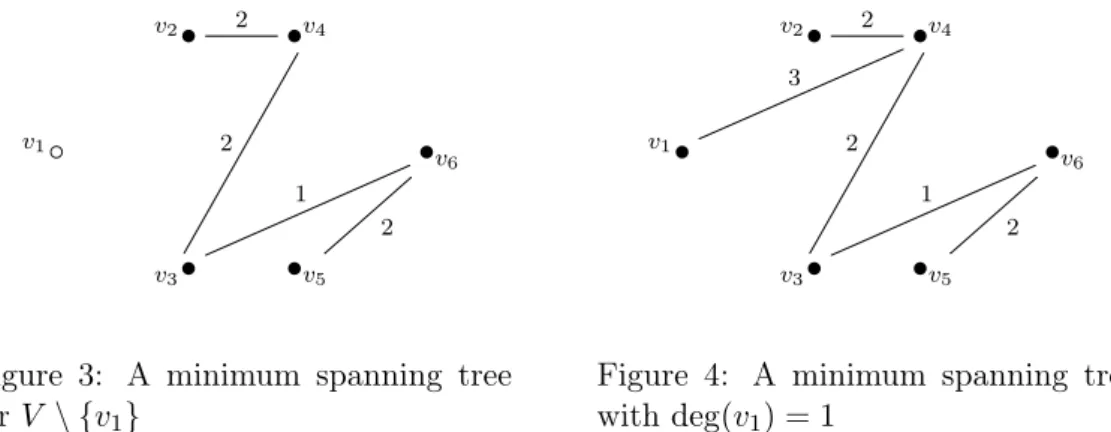
We want to find a minimum spanning tree with deg(v1) = 3. First of all it is necessary to set up a minimum spanning tree for the vertices V \ {v1} = {v2, . . . , v6}. With the classical algorithms for the (unconstrained) minimum spanning tree we get the pair vertices/edges
T = (V, S), whereV ={v2, . . . , v6}and S ={(v2, v4),(v3, v4),(v3, v6),(v5, v6)}. The tree is represented here below on the left.
v2• 2 •v4 v1◦ • v6 v3• 2 1 •v5 2
Figure 3: A minimum spanning tree for V \ {v1} v2• 2 •v4 v1• 3 •v6 v3• 2 1 •v5 2
Figure 4: A minimum spanning tree withdeg(v1) = 1
Now, by following the first step of Algorithm 3, (v1, v4) is a minimum edge incident in v1 and then we firstly updateS=S∪ {(v1, v4)}, roots:={v4}. The new tree is represented above on the right.
As|roots| 6= 3, we have to consider the nodesvsuch that(v1, v)exists withv /∈roots. These nodes arev2, v3, v5, v6. We have to compute for these nodes the “weights” c0(vi) =c(v1, vi)−c(e),
whereeis a maximum edge non incident in v1 in the pathvi. . . v0. We get
c0(v2) = c(v1, v2)−c(v2, v4) = 6−2 = 4
c0(v3) = c(v1, v3)−c(v3, v4) = 5−2 = 3
c0(v5) = c(v1, v5)−c(v5, v6) = 4−2 = 2
c0(v6) = c(v1, v6)−c(v3, v4) = 3−2 = 1
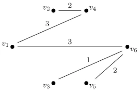
The vertex v6 is chosen and consequently the arc(v3, v4) is removed from the tree.
V ={v1, v2, . . . , v6} and S=S∪ {(v1, v6)} \ {(v3, v4)}. v2• 2 •v4 v1• 3 3 • v6 v3• 1 •v5 2
Figure 5: A minimum spanning tree withdeg(v1) = 2
As|roots| 6= 3, we have to consider again the nodesv such that(v1, v) exists withv /∈roots. These nodes are now v2, v3, v5. The weights are
c0(v2) = c(v1, v2)−c(v2, v4) = 6−2 = 4
c0(v3) = c(v1, v3)−c(v3, v6) = 5−1 = 4
c0(v5) = c(v1, v5)−c(v5, v6) = 4−2 = 2
The vertex v5 is chosen and consequently the arc(v5, v6) is removed from the tree.
V ={v1, v2, . . . , v6} and S=S∪ {(v1, v5)} \ {(v5, v6)}. A minimum spanning tree with deg(v1) = 3 is here below.
v2• 2 •v4 v1• 3 4 3 •v6 v3• 1 •v5
7
Some considerations on the computational complexity
Suppose G has n nodes. At each iteration of Algorithm 3 we must find, for each of the roots, the path that connects them to v0 and find in this path a maximum cost edge. This operation can be done easily if an orientation is given to the edges. We may think that in the tree every node has a depth, given by the number of edges in the only path that connects the node tov0: a node with depthiis a descendant of a node with depthi−1. For the purposes of Algorithm 3 it is important to know, for every node its (unique) predecessor, in order to get the path that connects it to a root.
Here is an algorithm that, with a fixed node v0, constructs an order of the nodes based on the depths in relation to the root.
begin
predecessors:={v0};
S:=set of the nodes of the tree; while predecessors6=∅ do
begin
descendants:=∅;
for eachx∈predecessors, if the edge(x, y)
exists in the tree andy∈S, then descendants:=descendants∪ {y}; pred(y) :=x; S:=S\predecessors; predecessors:=descendants; end end
Since the algorithm considers the nodes just once and for each of them the search for de-scendants can be performed innsteps, the algorithm terminates in at mostn2 steps. Once the nodes are sorted this way, the search for a maximum edge in the path connecting a root to v0 can be performed in at most n steps. Clearly after the removal of this edge the descendants have to be updated: the picture shows what can happen.
v0 r a t v u
Here r is a root and u and v are two possible roots. Suppose the algorithm decides on the basis of costs to add edge(v0, u)and remove edge a. At the next stepv no longer descend from
r but from u. We just need to reverse the order of descendants in the path u . . . t, that can be done in nsteps. Remembering that a minimum spanning tree can be found in O(n2) steps, Algorithm 3 for the search of a minimum spanning tree withdeg(v0) =k requiresO(kn2)steps to terminate.
8
Further developments and conclusions
It is known that the greedy algorithm, namely the way of “choosing the best” one step after the other, not always takes to the correct best final result. It depends on the kind of problem we have. Interesting connections with the so called matroid theory exist. We have seen that with the minimum spanning tree with one degree constraint, that is a degree constraint on one of the vertices of the graph, the technique works. It is interesting that if we consider a slightly generalised version of this problem, for example just the degree constraint on two of the vertices, the greedy technique does not work any more. We intend to consider this problem in the general context of degree-constrained minimum spanning tree in a future work.
References
[1] C. Papadimitriou, M. Yannakakis, The complexity of restricted spanning tree problems, Journal of the Associationn for Computing Machinery, Vol. 29, No. 2, 1982, pp. 285–309. [2] C. Papadimitriou, K. Steiglitz, Combinatorial optimization algorithms, Prentice–Hall,
En-glewood Cliffs, N.J., 1982.
[3] A.V. Aho, J.E. Hopcroft, J.D. Ullman, The design and analysis of computer algorithms, Addison–Wesley, Reading, Mass., 1974.