*Corresponding Author: Bahareh Jabalbarezi, M.Sc. Expert in Management of Desert, Faculty of Natural Resource, University of Tehran, Iran ([email protected])
A R T I C L E I N F O A B S T R A C T
Article history:
Received: 17 Jan 2017 Revised:29 Feb 2017 Accepted: 14 Mar 2017 ePublished: 30 Apr 2017
Key words: Artificial neural networks ANFIS model Soil temperature Levenberg Marquardt
Introduction
Soil temperature is found to be one of the most substantial climatic parameters in hydrological research. At the same time, soil moisture as a soil hydrologic parameter can be affected by soil temperature among others (Chu et al., 1988). Soil moisture content and volume in turn controls various hydrological processes (Alshorbag et al., 2008). Given the enormous studies on
role of soil temperature in agricultural studies, engineering applications (Chu et al., 1988) and hydrological modeling and etc. demonstrated that, it seems necessary to emphasize importance of understanding the changes in soil temperature. In lights of previous literatures, soil temperature and moisture variations at shallow depths demonstrates significant fluctuations in daily and in annual scale. So it is difficult International Journal of Advanced Biological and Biomedical Research 5(2) (2017) 52–59
Journal homepage: www.ijabbr.com
Research Article
DOI: 10.18869/IJABBR.2017.419
Potential Assessment of ANNs and Adaptative Neuro Fuzzy Inference systems (ANFIS) for
Simulating Soil Temperature at diffrent Soil Profile Depths
Marjan Behnia1, Hooshang Akbari Valani1, Moslem Bameri2, Bahareh Jabalbarezi*1, Hamed Eskandari Damaneh3
1M.Sc. Expert in Management of Desert, Faculty of Natural Resource, University of Tehran, Iran
2M.Sc. Expert in De-Desertification, Faculty of Agriculture and Natural Resource, Hormozgan university, Iran 3PhD Student of De-Desertication, Faculty of Natural Resource, University of Tehran, Iran
to predict the soil temperature. Considering the soil temperature changes in numerical methods that can accurately predict thermal behavior of soil to assess changes in soil temperature over time can be useful for the purpose of agricultural activities. Many different methods such as artificial neural networks (Yang et al., 1997), statistical techniques and Contingency analysis (Bouk et al., 1974; Conrad et al., 1950; Han et al., 1977) have been used to model the soil temperature. Yang et al (1997) applied artificial neural networks to simulate the soil temperature at various depths of 100, 500 and 1500 mm, in an Experimental Farm in Ottawa, Canada. Results using two criteria root mean square error (RMSE) (0.59 to 1.82) and correlation coefficient (0.93 to 0.98) reflects the efficiency of artificial neural networks to estimate soil temperature. Kang et al (2000) applied soil temperature hybrid model taking into account the combined effect of topography, vegetation and litter to predict the soil temperature in forest areas in Korea. Sensitivity analysis of model showed high sensitivity to leaf area index (LAI). Kuaho et al (2009) by integrating radial neural networks and clustering methods, simulated the soil profile temperature. Their results indicated that the combination of these two methods has high potential in determining the thermal behavior and soil moisture in different depths. The models which are based on monthly or yearly series may not be able to correctly predict dynamic variations in soil temperature, so measuring daily soil temperature in each zone is very important. On the other hand, measuring soil temperature for a long-term is difficult and very expensive (kiosk et al., 1997). Hence this study aims to study and estimate the soil temperature using time series models and multivariate regression methods. Fuzzy Logic is one of Artificial Intelligence method which synthesis human knowledge with observational data to create fuzzy rules and Fuzzy Inference System (Zadeh 1965). A Fuzzy Inference System, convert a set of inputs to numeric outputs using fuzzy rules and membership functions. Fuzzy inference systems serve as effective method for modeling complex systems that cannot be simulated them with conventional statistical methods. Artificial neural network and fuzzy inference systems Methods are increasingly being used to model the rainfall-runoff hydrological processes, including modeling, simulation and prediction of flood, etc. among others. However, one of the main variables that play a role in hydrological studies and estimating evapotranspiration and soil temperature of the stream that has been less studied and modeled. The present research attempts using artificial neural network and
fuzzy inference systems simulate soil temperature at a depth 5 to 100 cm soil temperature simulation and to assess their efficiency in modeling.
Materials and Methods
In doing present research, climatic parameters from Isfahan synoptic meteorological station including the average daily air temperature, minimum and maximum daily temperatures, evaporation, solar radiation, soil temperature and sunshine hours in the middle of the 5, 10, 20, 30, 50 and 100 cm during the 13 year period (1992-2009) as an arid and semi-arid region of the country and with moderately severe seasonal weather changes were collected. The study area is shown in Figure 1.
Figure 1: Study area map
The data were divided into two parts. First part included 3028 observational data to train models and 335 observational for data validation models were used. Two standard assessment correlation criteria (R2) and the average root mean square error (RMSE) were used to model validation.
Given that input parameters are characterized with different scale, so before entering the model in a certain numerical range were standardized. Using following formula all entries were scaled in range -1 to +1. Such inputs scaling are also effective to enhance performance tangent sigmoid function in neural networks. The following function was used to scale inputs and outputs before entering the artificial intelligence models.
1
)
(
)
(
*
2
min max
min
X
X
X
X
Where, is standardized value Z between -1 and +1 and Xmin and Xmax is the minimum and maximum input and output respectively.
ANFIS modeling
ANFIS for first time was coined by Jang (1993). A fuzzy system with algorithm that is based on neural network theory should be trained. The combination of artificial neural networks and fuzzy logic systems based on neural network as fuzzy inference system has comparative advantages in computational framework. The ability to effectively train artificial neural networks and fuzzy if-then rules can contribute parameter optimization (Nayak et al., 2004).
Fuzzy Logic
Fuzzy Logic was presented for the first time by Lotfi Zadeh (1965). This powerful and flexible utility theory to model the input data to output data. The primary mechanism of input and output data modeling is to determine the terms commonly called laws. Modeling based on fuzzy rules is a form of quantitative modeling where behavior of the system using a natural language is described (Nayak et al., 2004). All rules are evaluated for synchronous and parallel rank is not important rules. Rules relating to the functions and variables that explain those variables. There are two types of systems that are widely used fuzzy rules, and these two types by Namdani and Assilian (1974) is presented. The method used in this research is Takagi-Sugeno. This method is a combination of fuzzy logic and fuzzy process output to be working. In general, a fuzzy system consists of several details that include: phase of the inputs, the use of a fuzzy operator, applying a conceptual approach, combining the output and the defuzzification.
Fuzzification
Each node of this layer using the membership function, sets score each entry according to the appropriate fuzzy.
2
1,
2,
1, 2 ( )
3, 4 ( )
i
i
i A
i B
i O x
i O x
Where x and y represents non-fuzzy inputs to ith node
and
A
i andB
i2 denotes linguistic labels characterizedwith
Aiand
B2respectively. In this study, thefollowing formula is used with Gaussian fuzzy. 2
( ; , ) exp x c
Gaussmf x c
In this regard, c is center and
represents membership function width are nonlinear adjustable variables calculated by the system.Rule nodes
In this layer the operator "and" is used to obtain output
that represents the front section of the law. Hence (
O
2,k)outputs is multiplication of degree to first layer.
2,k Ai( ) Bi( )
O
x
yWeighting and normalization
The main purpose of this layer is to determine ith weight of (wi) than the sum of the law.
4 3, 1 i i i k k w Q w w
Defuzzification
Phase outputs are explicit. This means that real values of membership functions and its relation to the real number is obtained and is considered as linear factor of proviso.
4,i i i i( i i i)
O w f w p x q y r
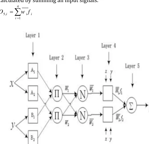
In this layer there is a node, the overall output is calculated by summing all input signals.
4
5, 1
i i i
i
O w f
Figure 2. ANFIS model structure
Subtractive clustering
Subtractive clustering algorithm is used to reduce the dimensionality of data in cases where a large number of inputs exist, depending on the input data. Using foregoing algorithm fuzzy system can be organized with the least number of fuzzy rules. Subtractive clustering depends on the data density. Considering n data points {x1, ..., xn}, subtractive clustering algorithm considers each point as a potential cluster center. Then density index at point xi is defined as follows:
n j a r j x i x ie
D
1 2 2 / / 2has more neighborhoods points has more potential to get on the cluster centers.
Observational data that are located outside the radius impose less impact on density index. Selecting clustering radius is of great importance in determining the number of clusters. High values ra result in a lower number of clusters and vice versa. After a point with the highest potential was determined as cluster center, for example xc1 point was determined as first center of the cluster by Dci density index for each point xi will be recalculated by following formula.
/2
2/ 2
1 rb
c x i x i c i
i
D
D
e
D
Where rb is a positive constant greater than zero (rb> 0) and represents the neighborhood radius for which the greatest reduction in the density will be achieved. To avoid proximity of cluster centers to each other usually rb is set as much as 1.5 times of ra.
Finally data clusters are used to determine the number of fuzzy rules used in the fuzzy inference system.
Artificial Neural Networks
Artificial neural networks are different from conventional systems such as statistical or analytical models Mitt different weight to input from other nodes receives, responds. So far, different neural networks with different algorithms have been used in hydrological studies. Artificial neural networks are different from conventional systems such as statistical or analytical models. An artificial neural network consists of an arbitrary number of very simple elements which are called nodes. Each node is a very simple element with different weights processor that inputs received from other nodes-the-answers. So far, different neural networks with different algorithms have been used in hydrological studies. In the present research feed forward networks MLP propagation learning method was used. The reason behind selecting this type of artificial neural networks is that in previous research, this type of network performance outperforms other types of neural networks in the field of hydrology and water resources (Cigizoglu and Alp, 2008).
Results and Discussion
Table 1 illustrates the demographics series of parameters used in the study. As it can be seen, coefficient of variation (Cv) from surface to a depth of 100 cm soil temperature has increased substantially so that maximum coefficient of variation of soil temperature is observed at a depth of 5 cm and decreases with depth
gradually. High values of the coefficient of variation of soil surface layers suggest high variability in soil temperature in this layer, which in turn is influenced by a variety of mechanisms in soil temperature in this layer. Artificial neural network techniques and Fuzzy Inference System methods was used to simulate soil temperature at different depths. To simulate soil temperature at depths 5 to 100 cm, six artificial neural network model and six ANFIS model were used. To achieve the appropriate structure Artificial neural network trial and error process to achieve the most appropriate structure based on determining neural network the number of hidden layer neurons.
Number of neurons in the hidden layer is determined given to number of model inputs. Usually the number of hidden layer neurons is determined between 1 to 2m + 1based on trial and error, where m is the number of inputs. To determine artificial neural network the Levenberg-Marquardt and 300 training rounds were used.
The most appropriate number of neurons in the hidden layer to simulate the soil temperature in layers 5, 10, 20, 30, 50 and 100 cm, were set as, 3, 4, 5, 4, 5, and 3 neurons respectively.
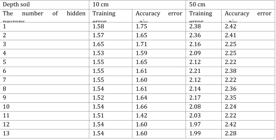
For example, Table 2 shows the trial and error for artificial neural network model to depths of 10 and 50 cm.
Table 1. Descriptive statistics for soil temperature series
Variable Descriptive statistics
min max Avge sd skewness Kurtosis CV (%)
Input variables
(Co) Temprature min -7.8 28.80 13.04 7.14 -0.39 -0.73 54.77
(Co) maximum air temperature
1.2 43 28.53 8.20 -0.60 -0.51 28.76
(CAL/CM2)radiation 25 969.5 1845.67 1122.42 1.38 8.49 60.81
(hr)sunny hours 0.1 13.8 9.98 2.75 -1.65 2.74 27.56
(mm)evaporation 0.1 30 8.11 4.12 -.02 -0.48 50.83
(Co)average temprature -3.30 34.80 20.78 7.50 -0.48 -0.73 36.33 output
variables
5 cm(Co) 0.70 45.53 26.24 9.69 -0.48 -0.89 36.94
10 cm(Co) 0.30 39.67 25.73 9.16 -0.56 -0.79 35.61
20 cm(Co) 2.07 36.67 24.31 8.01 -0.58 -0.79 32.95
30 cm(Co) 3.40 37.13 24.05 7.63 -0.56 -0.86 31.72
50 cm(Co) 7.33 35 24.37 6.62 -0.53 -0.92 27.14
100 cm(Co) 10.60 32.93 23.59 5.08 -0.50 -0.92 21.52
Table 2: Determination of artificial neural network model structure to depths 10 and 50 cm using a trial and error process
Depth soil 10 cm 50 cm
The number of hidden neurons
Training error
Accuracy error یجنس
Training error
Accuracy error یجنس
1 1.58 1.75 2.38 2.42
2 1.57 1.65 2.36 2.41
3 1.65 1.71 2.16 2.25
4 1.53 1.59 2.09 2.25
5 1.55 1.65 2.12 2.22
6 1.55 1.61 2.21 2.38
7 1.55 1.60 2.12 2.22
8 1.54 1.61 2.14 2.36
9 1.52 1.64 2.17 2.35
10 1.54 1.66 2.08 2.24
11 1.51 1.42 2.03 2.22
12 1.54 1.60 1.97 2.42
13 1.54 1.60 1.99 2.28
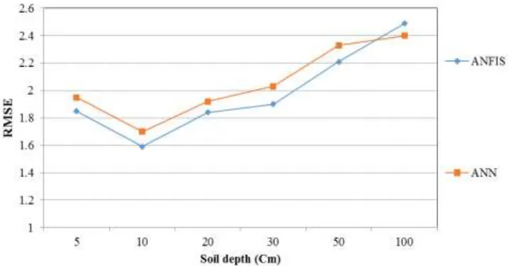
Table 3: The results of ANN and ANFIS models to simulate the temperature at different depths
ANFIS ANN
Depth(cm) R2 RMSE (Co) R2 RMSE(Co)
5 0.98 1.86 0.98 1.95
10 0.98 1.58 0.98 1.59
20 0.96 1.84 0.96 1.92
30 0.95 1.89 0.89 2.03
50 0.91 2.15 0.91 2.22
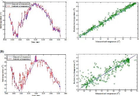
Figure 2 and 3 illustrate correlation graph for observational data and simulation data using ANFIS model and artificial neural network. According to the graphs it is clear that both ANFIS and artificial neural network model have been successful in simulating soil temperature. Here, for example, ANN and ANFIS models simulation results in depths 5 and 100 cm are given. As
for Figures 2 and 3 it is worthy to note that agreement between observed and simulated data in surface layers than deeper ones is higher which representing higher efficient models used in the surface layers than deep layers.
Figure 4: ANN model potential to simulate soil temperature data in depth (A) 5 cm and (b) 100 cm
Figure 5: ANFIS model potential to simulate soil temperature data in depth (A) 5 cm and (b) 100 cm
The results of ANN and ANFIS models to simulate different depths of soil temperature are shown in Figure 4. According to the figure that both model error increases with increasing depth and the maximum depth of 100 cm and the lowest error model error models at a depth of 10 cm from the surface. The results in Table 3 also represents an increase of artificial neural network models and ANFIS error in the simulated temperature changes in the soil is deep layers. So that the minimum and maximum error (RMSE) for ANFIS and artificial neural network models are 1.86 and 1.95 respectively (at depth 5 cm) and 2.39 and 2.44 (at depth 100 cm). On the other hand comparing simulation results of ANFIS model in Figure 3 and artificial neural network in Figure 4 as well as the results set forth in Table 3 suggested superior efficiency of the artificial neural network than ANFIS model. The main reason for increasing the effectiveness artificial intelligence models in simulating soil temperature in the surface layers than depths is mainly
Concluding Remarks
Soil temperature represents one of the key variables in natural resources research, especially hydrological studies and estimation of hydrologic characteristics as streams and evapotranspiration. In this study, artificial neural network models and Fuzzy Inference System (ANFIS) was used to simulate soil temperature in different layers. The result represents coefficient of variation of soil temperature in the surface layers than upper layers. The main objective aims to shed lights on potential of artificial neural networks (ANNs) and Neuro-Fuzzy inference system (ANFIS) to simulate soil temperature at 5-100 cm depths. The ANNs structure was designed by one input layer, one hidden layer and finally one output layer. The network was trained using Levenberg-Marquardt training algorithm, then the trial and error was considered to determine optimal number of hidden neurons. The main reason for increasing the effectiveness artificial intelligence models in simulating soil temperature in the surface layers than depths is mainly related to a decrease in the correlation between climate and soil temperature changes in the deep layers than upper ones so that the coefficient of variation of soil temperature with increasing depth is less than surface layers and is less affected by climatic variables including soil temperature. Increased accuracy of artificial neural network models and ANFIS in the surface layers stems from complex relationships between climatic variables and soil temperatures in the surface layers. Although the obtained results suggests an increase in the efficiency of ANFIS model to artificial neural network in different soil layers, however, it merits much more investigations to compare artificial neural networks and ANFIS in simulating soil temperature under different climatic conditions to get a comprehensive conclusion in this field.
References
Bocock, K. L., Lindley, D. K.,Gill, C. A., Adamson, J. K. and Webster, J. A. 1974. Harmonic analysis and synthesis: Basic principles of the technique and some applications to temperature data Mercewood Res. Dev. No.54.
Chio, J. S., Fermanian, T. W., Weh ner, D. J. and Spomer, L. A. 1988. Effect of temperature, moisture and soil texture on DCPA degradation. Agron. J. 80: 108-11.
Cigizoglu, H. K., Alp, M., (2008), “Generalized Regression Neural Network in Modeling River Sediment Yield”, J. of Advances in Engineering Software, 37, pp 63-68.
Coelho, L. D., Freire, R. Z., Santos, G. H. D., Mendes, N. 2009. Identification of temperature and moisture content fields using a combined neural network and clustering method approach, International Communications in Heat and Mass Transfer. doi:10.1016/j.icheatmasstransfer.2009.01.012.
Conard, V. and Pollock, L. W. 1950. Methods in climatology, Harvard Uni. Press, Cambridge Mass:119-133.
Elshorbagy, A. and Parasuraman, K., 2008. On the relevance of using artificial neural networksfor estimating soil moisture content. J Hydrol. 362, 1– 18.
Gao, Z., Bian, L., Hu, Y., Wang, L. and Fan, J., 2007. Determination of soil temperature in an arid region. J Arid Environ. 71, 157-168.
Hann, C. E. 1977. Statistical methods in hydrology. Iowa State univ. Press.
Jang, J.S.R., 1993. ANFIS: Adaptive network based fuzzy inference system, IEEE Trans. On System, Man, and Cybernetics, 23(3): 665-685.
Jenkins, G. M. 1976. Time series analysis, forecasting and control, revised edn. Holden-Day, San Francisco.
Kuuseokes, E., Liechty, H. O., Reed, D. D. and Dong, J. 1997. Relating site specific weather data to regional monitoring networks in the late states. For. Sci. 43: 447-452.
Mamdani, E.H. and Assilian, S., 1975. An experiment in linguistic synthesis with a fuzzy logic controller. International Journal of Man-Machine Studies, 7(1): 1-13.
Nayak, P.C., Sudheer, K.P., Rangan, D.M. and Ramasatri, K.S., 2004. A neuro-fuzzy computing technique for modeling hydrological time series. Journal of Hydrology, 291: 52-66.
Yang , C. C., Parsher, S. O., Mehuys, G. R. and Panti, N. K. 1997. Application of artificial neural networks for simulation of soil temperature. Agric. Eng 40(3): 649-656.
Zadeh, L.A., 1965. Fuzzy sets. Information Control, 8, 338– 353.