*Corresponding author: [email protected] 2018 UTHM Publisher. All right reserved.
e-ISSN: 2600-7924/penerbit.uthm.edu.my/ojs/index.php/jst
Performance Evaluation of Feed Forward Neural Network for Image
Classification
H. Ullah
1,2*, M.A. Kiber
1, A.H.M. A. Huq
1and M.A.S. Bhuiyan
31Electrical and Electronic Engineering, University of Dhaka, Bangladesh. 2Electrical and Electronic Engineering,Southern University Bangladesh, Bangladesh.
3Electrical and Electronics Engineering, Xiamen University Malaysia, Malaysia. Received 30 January 2018; accepted 29 April 2018; available online 19 May 2018
1. Introduction
Learning-based techniques have captured a wide range of consideration for pattern recognition or classification problems. NN models are indicated to achieve high performance compared to other existing models in many recognition or classification works [1]. ANN is a network of neurons which is preferred because of its dynamic nature. The merits of neural network come from its ability for recognizing and nonlinear relationships of model among data. So, ANNs have many applications as the intelligent modeling techniques [2] and are the easiest way for dealing nonlinear relationships and clustering of real data compare to strict linear relationship [3]. But ANNs designers face two problems, one is the network structure and another is the network generalization. ANNs design needs application-specific appropriate architecture that includes network type, number of layers, number of neurons in hidden layers, and activation functions between layers. A single-input neuron and a multiple-input neuron are shown in Fig. 1. Here, the scalar input is multiplied by the scalar weight and the other input is multiplied by a bias or offset. The summer output often referred to as the net input which goes to the transfer
function (activation function)that produces the scalar neuron output. The neuron output is calculated by a=f (wp+b). The actual output depends on the specific activation function that is chosen. The bias is almost like a weight except that it has a constant value of 1. Generally, a neuron has more than one input. A neuron with R inputs is shown in Fig. 1(b). The individual inputs p1,p2,p3,..., pR are each weighted by corresponding elements w1,1, w1,2,w1,3...,w1,R of the weight matrix W.
(a) (b)
Fig. 1: (a) single-input neuron, and (b) multiple-input neuron.
The transfer function can be a linear or a nonlinear function of n. A particular transfer function is chosen to satisfy some specific purposes of the problem so that the neuron is trying to solve. There are a lot of transfer functions. Four of them are commonly used transfer functions for different purposes. These are log sigmoid, tan sigmoid, pure linear and Abstract: Artificial Neural Networks (ANNs) are one of the most comprehensive tools for classification. In this study, the performance of Feed Forward Neural Network (FFNN) with back-propagation algorithm is used to find out the appropriate activation function in the hidden layer using MATLAB 2013a. Random data has been generated and fetched to FFNN for testing the classification performance of this network. From the values of MSE, response graph and regression coefficients, it is clear that Tan sigmoid activation function is the best choice for the image classification. The FFNN with this activation function is better for any classification purpose of different applications such as aerospace, automotive, materials, manufacturing, petroleum, robotics, communication etc because to perform the classification the network designer have to choose an activation function.
Keyword: Activation Function; ANN; Back-Propagation Algorithm; FFNN; Regression.
20
hard limit activation function and explained them below:
1. Log Sigmoid: This transfer function takes the input (which may have any value between plus and minus infinity) and squashes the output into the range 0 to 1, according to the following expression:
x e 1 1 f(x) (1)
The log-sigmoid transfer function is commonly used in multilayer networks that are trained using the back-propagation algorithm.
2. Tan Sigmoid (Hyperbolic Tangent Sigmoid): This is another important transfer function that is also huge used in the multilayer networks. The expression of this transfer function is given in below:
1 1 f(x) 2 2 xx
e e
(2)
3. Pure Linear: The output of a linear transfer function is equal to its input that is a=n [f(x)=x]. Neurons with this transfer function are used in the ADALINE networks. The output versus input characteristic of a single-input linear neuron with a bias.
4. Hard Limit: The hard limit transfer function that is set the output of the neuron to 0 if the function argument is less than 0 and 1 if its argument is greater than or equal to 0.
Many studies had been carried out on artificial neural networks for classifying purposes. Based on studies, ANNs are categorized as FFNN, Cascade-Forward Neural Network, Nonlinear Auto-Regression Neural Network, Generalized Regression Neural Network (GRNN), Recurrent Neural Network (RNN), Radial Basis Function Neural Network (RBFNN) and Probabilistic Neural Network (PNN)[4]. All these are application specific. As the examples, Gao (2017) is designed an algorithm with higher classification accuracy for cloud security intrusion detection using GRNN[5]. Zia et al.(2017) have proposed a method with high performance and best recognition rate for piano’s continuous note recognition by RNN [6]. Yu et al. (2017) have proposed a concept to pump the oil using RBFNN combined with
modified Genetic Algorithm with good convergence performance, high accuracy, and high reliability [7]. Mao et al. (2000) has designed an algorithm for pattern classification with Genetic Algorithm by PNN with with satisfactory classification accuracy [8]. For classification purpose, FFNN with back-propagation learning algorithm, also known as a Feed-Forward Back propagation neural network (FFBPNN) is usually preferred because of its high accuracy and less iterations period [9]. It is very simple and effective model of ANNs where a lot of input and target pairs are required for training and testing phases [10]. As it works only in multilayer, so it is also called multilayer FF neural network [11]. There are different types of training algorithm in NN such as Gradient Descent, Conjugate Gradient, Newton's Method, Quasi-Newton's Method and Train Levenberg Marquartdt Algorithm (LMA). Corte-Valiente et al. (2017) evaluates the performance of these types of training algorithms in a FFNN for analyzing the whole uniformity in the lighting systems of outdoor and they found the minimum error with LMA [12].
Dhande and Gulhane (2012) developed a classifier of FFNN with back propagation algorithm for patients survival analysis and found that it has better accuracy compared to Radial Basis Function Neural Network (RBFNN) [13]. Narula and Kaur (2015) designed a fuzzy-feed forward back-propagation neural network technique for retrieving the medical images and showed that it retrieves 100% precision and better recall values than other techniques [14]. Yongming Wang and Junzhong Gu (2014) compare the performance of FFBPNN, RBFNN and GRNN and found that the performance of FFBPNN is better compare to others two in term of Mean Absolute Error (MAE), Root Mean Square Error (RMSE) and the coefficient of determination (R2) [15]. J. Pradeep et. al. (2012) designed a neural network(FFBPNN) based recognition system integrating feature extraction and classification for english handwritten and found that it is more less complex and allows faster recognition system compared to other neural networks [16].
21
based on attributes of that object. There are many real world applications that can be categorized by classification problems such as weather forecast, credit risk evaluation, medical diagnosis, bankruptcy prediction, speech recognition, handwritten character recognition [17]. The training of neural network is a complex task in this field of research. The main difficulty for adopting ANN is to find the appropriate combination of learning, transfer and training functions for the classification. In this paper, the performances of the four transfer functions (log sigmoid, tan sigmoid, pure linear and hard limit) in FFBPNN with trial and error approach will be determined to find out the best activation function for identifying the output classification responses of this network with two input and four output features (classes).
2. Methodology
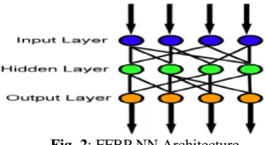
FFNN with back propagation algorithm (FFBPNN) has the better accuracy and precision compared to than other techniques for classification application. FFBPNN computes output in forward and error in backward direction. In forward processing, Input layer is used for taking the input data that is passed on to the hidden layers, and hidden layer processes the data. Output is taken from the output layer which is shown in Fig. 2. FFNN with back propagation training is the most commonly used technique for training the ANN to minimize the gradient. For this research, Neural Network Toolbox™ of MATLAB (Version 2013a) has been used.
Fig. 2: FFBP NN Architecture
The design algorithm of this network for classification is as follows:
Step 1. Generate the data Step 2. Create the network Step 3. Configure the network
Step 4. Initialize the weights and biases randomly
Step 5. Train the network
Step 6. Propagate the inputs to the forward Step 7. Back propagate the error to the hidden layer
Step 8. Validate the network
Step 9. Use and analysis the performance of the network.
At first random data has been generated to prepare training data which is introduced to this network as input and target vectors for testing the classification performance. Then the network is created and configured by the relevant matlab function, where the weights and biases are initialized randomly. The network is trained by another appropriate matlab function and after training, the inputs are propagated to the forwarded and output is calculated in forward direction. The performance error is calculated in backward direction. At first the initial number of neurons, layers, and activation function are found out, and the error of performance is recorded. In the case of two-hidden-layer with m output neurons, the number of hidden nodes that are enough to learn N samples with negligibly small error for this network can be calculated by the following equations[18]:
N
m
2
)
(
2
(3)Specifically, it is suggested that the sufficient number of hidden nodes in the first layer is:
N
m
m
N
/(
2
)
(
2
)
2
(4)and in the second it is:
)
2
/(
m
N
m
(5)and also the activation function for this networ, Ai is equal to
N i i j j ii w x b
A
1
(6)
Where 𝑁 is the amount of elements of input vector, 𝜔𝑖𝑗 are the interconnection
22
bias is the coefficient that controls the transfer of the signal followed by this network [4]. After that for the same architecture, the activation function type is changed and the error of performance is also recorded. This procedure is repeated to identify the best activation function based on MSE of performance graph, regression co-efficient, response graph, classified graph and histogram error graph and information is recorded. Based on this algorithm, the architecture of this network including input, output and hidden layers is shown in Fig. 3.
Fig. 3: The FFNN architecture
3. Simulation Result and Discussion
In this work, Neural Network Toolbox™ of MATLAB (Version 2013a) has been used. The data is generated randomly which is divided into three categories: training data, validation data and test data with ratio 75:15:10 respectively. The Performance graph is counted in terms of mean square error. The numbers of neurons for the two successive hidden layers are six and three respectively. The number of input layer nodes is two which describes the input features and the number of output layer nodes is four that also describes the target (output) classes. The activation function in the output is pure linear (by default). In this work, the appropriate activation function in the hidden layers will be determined by evaluating the MSE of performance graphs, response graph, regression co-efficient values, etc and simulation is conducted five times and the better result is counted from this.
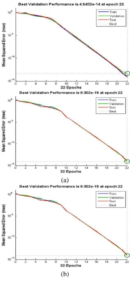
Fig. 4 shows the MSE of performance graph for four different activation functions. From this figure, it is shown that the performance error for the tan sigmoid function is the least (8.302e-15) and the performance error for the hard limit function is high (0.46025). So the best activation function is tan sigmoid and the worst activation function is hard limit of FFBPNN for any recognition applications.
The network response graphs for the four activation functions are shown in Fig. 5. From this figure, it is clear that the response graph for the Tan sigmoid activation function is almost same with the target and for the Log sigmoid activation function; it is a little bit different from the target but for the Pure Linear and hard Limit is completely abrupt from the target. So, from this scenery it is evident that Tan Sigmoid function is better than other activation functions.
(a)
23
(c)
(d)
Fig. 4: The Performance graphs for the (a) Log Sigmoid, (b) Tan Sigmoid, (c) Pure Linear, and (d) Hard Limit activation function.
(a)
(b)
(c)
(d)
Fig. 5: The network response graphs for the (a) Log Sigmoid,(b) Tan Sigmoid, (c) Pure Linear, and (d) Hard Limit activation function for any iteration.
24
(a)
(b)
(c)
(d)
Fig. 6: The classified graphs for the (a) Log Sigmoid, (b) Tan Sigmoid, (c) Pure Linear, and (d) Hard Limit activation function for any iteration.
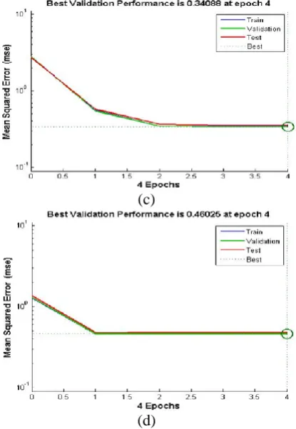
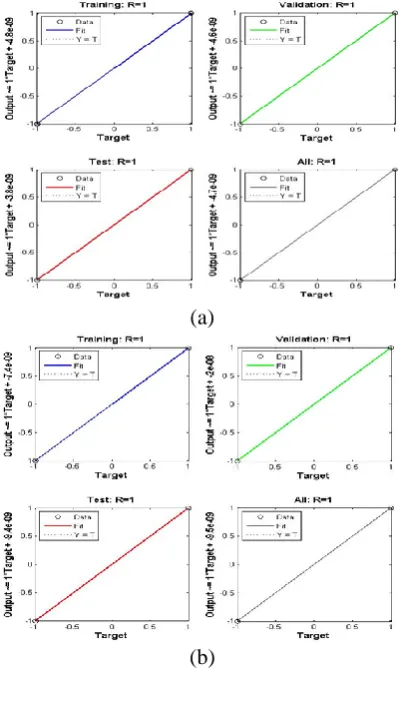
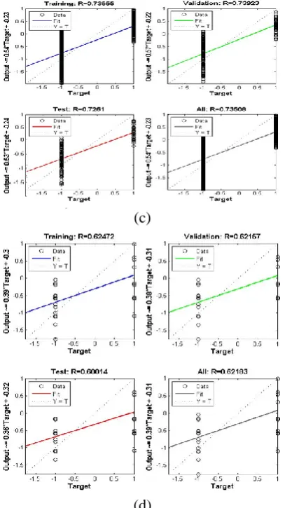
Regression plot is another most important feature for verifying the network performance as shown in Fig. 7. For the best fitting of data by this network, the desired value of Regression co-efficient (R) is equal to 1 and its value near to 0 is completely undesirable. The Regression plot [19] represents the relationship between input and output parameters which is given by the following equation: Output= learning-rate × target + bias.
From the regression plot, it is clear that the regression plot for the target and fitting data is almost similar for the log sigmoid and tan sigmoid activation function, where the value of R is close to 1 for both. Therefore, the networks by these activation functions have fit the data well after training. The regression plot for the fitting data is huge diverse form the target data plot for the other activation functions.
(a)
25
(c)
(d)
Fig. 7: Regression plots for the (a) Log Sigmoid, (b) Tan Sigmoid, (c) Pure Linear, and (d) Hard Limit activation function.
The histogram error graph is shown in Fig. 8. From these graphs, it is observed that the most of the errors of instances is near to zero and only a few instances of the errors is away from zero for the log sigmoid and tan sigmoid activation function that is the desired for a good network. On the other hand for the pure linear and hard limit activation function, the error of instances is diverse from 0.
From the above illustrations, it is obvious that log sigmoid & tan sigmoid activation functions are better for the classification purpose compare to other two activation functions. But from the MSE of performance graphs (Fig. 5) and response graphs (Fig. 6), it is observed that the performance of tan sigmoid is the best suit compare to log sigmoid activation function. Therefore, tan sigmoid activation function of FFNN with back propagation algorithm is suggested in classification application for this kind of input data features.
(a)
(b)
(c)
(d)
26
Conclusion
From this research, it is evident that FFBPNN with tan sigmoid activation function can be used as a highly effective tool for any classifying purpose for getting the well performance with less traning time and complexity. It is also observed from the classifying and histogram graphs and also regression plots that performance of all activation functions is almost same but from the MSE and response graphs it is clear that tan sigmoid is better to choose as the activation function for a disigner during desigining the FFNN. From the network response graphs, it is becoming difficult to find out either log or tan segmoid activation function is better because we did not get any decimal values from this, graphical representation is the only basis and the difference of graphs for these activation functions is also too much small. But from the MSE performance graph, we got the dicimal vaue with the graphical representation so it is becomed easy for us to decide what activation function is better compared to others. Finally, we can also say that MSE is the best parameter to find out the best activation function.
References
[1] Fereidunian, A.R., Lesani, H. and Lucas, C. (2002) “Distribution System Reconfiguration using Pattern Recognizer Neural Networks”, International Journal of Engineering, Transaction B: Applications, Vol. 15, No. 2, pp. 135-144. [2] Neshat, N. (2015) “An approach of
artificial neural networks modeling based on fuzzy regression for forecasting purposes”, International Journal of Engineering-Transactions B: Applications, Vol. 28, No. 11, pp. 1651-1655.
[3] Naguib, R.N. and Sherbet, G. V. (2001) “Artificial neural networks in cancer diagnosis, prognosis, and patient management”, CRC Press LLC, New York, pp. 212-213.
[4] Haykin, S.(2005), “Neural Networks: A Comprehensive Foundation (Second Edition)”, Pearson Prentice Hall, London. [5] Gao, F. (2017) “Application of
Generalized Regression Neural Network in Cloud Security Intrusion Detection”, IEEE
2017 International Conference on Robots and Intelligent System, China.
[6] Jia, Y., Wu, Z., Xu,Y., Ke, D., and Su, K.(2017) “Long Short-Term Memory Projection Recurrent Neural Network Architectures for Piano’s Continuous Note Recognition”, Journal of Robotics, Vol. 2017, pp.1-7.
[7] Yu, D., Li, Y., Sun, H., Ren, Y., Zhang,Y., and Qi, Y. (2017) “A Fault Diagnosis Method for Oil Well Pump Using Radial Basis Function Neural Network Combined with Modified Genetic Algorithm”, Journal of Control Science and Engineering, Vol. 2017,pp.1-7.
[8] Mao, K. Z., Tan, K. C. and Ser, W. (2000) “Probabilistic Neural-Network Structure Determination for Pattern Classification”, IEEE Transactions On Neural Networks, Vol. 11, No. 4, pp.1009-1016.
[9] Rani, N. and Vashisth, S. (2016) “Brain Tumor Detection and Classification with Feed Forward Back Propagation Neural Network”, International Journal of Computer Applications, Vol. 146, No. 12 ,pp. 1-6.
[10] Amardeep, R. and Swamy, K. T. (2017), “Training Feed forward Neural Network With Backpropogation Algorithm”, International Journal of Engineering And Computer Science, Vol. 6, No. 1, pp. 19860-19866.
[11] Rodan, A., Faris, H. and Alqatawna, J. (2016) “Optimizing Feed-forward Neural Networks Using Biogeography Based Optimization for E-Mail Spam Identification”, Int. J. Communications, Network and System Sciences, Vol. 9, No. 1, pp. 19-28.
[12] Valiente , A. D. C., Sequera , J. L. C., Martinez , A. C., Pulido, J. M. G. and Martinez, J. M. G.(2017) “An Artificial Neural Network for Analyzing Overall Uniformity in Outdoor Lighting Systems”, Energies, Vol. 10, No. 2,pp. 1-18.
[13] Dhande, J. D. and Gulhane, S.M.(2012) “Design of Classifier Using Artificial Neural Network for Patients Survival Analysis”, International Journal of Engineering Science and Innovative Technology, Vol. 1, No. 2, pp. 278-282. [14] Narula, S. and Kaur, Er. S.(2015)
27
Journal of Engineering Development and Research, Vol. 3, No. 2, pp. 1224-1232. [15] Wang, Y. and Gu, J.(2014)
“Comparative study among three different artificial neural networks to infectious diarrhea forecasting”, IEEE International Conference on Bioinformatics and Biomedicine, Belfast, UK, pp. 40-46. [16] Pradeep, J., Srinivasan, E. and
Himavath, S.(2012) “Neural Network Based Recognition System Integrating Feature Extraction and Classification for English Handwritten”, Journal of Engineering, Transactions B: Applications,Vol. 25, No. 2, pp. 99-106. [17] Zhange, G. P.(2000), “Neural
Networks for Classification: A Survey”,
IEEE Transactions on Systems, Man, and cybernetics-part C: Applications and Reviews, Vol. 30, No. 4, pp. 451-462. [18] Huang, G. B. (2003). Learning
capability and storage capacity of two-hidden-layer feed-forward networks. IEEE Transactions on Neural Networks,Vol. 14, No. 2, pp. 274–281.