http://www.sciencepublishinggroup.com/j/ijics doi: 10.11648/j.ijics.20170203.11
Design of Single Phase Transformer Through Different
Optimization Techniques
Raju Basak
1, *, Hamed Yahoui
2, Nicolas Siauve
21GEP Department, University Claude Bernard Lyon1, Lyon, France 2Ampere Laboratory, University Claude Bernard Lyon1, Lyon, France
Email address:
[email protected] (R. Basak), [email protected] (H. Yahoui), [email protected] (N. Siauve) *Corresponding author
To cite this article:
Raju Basak, Hamed Yahoui, Nicolas Siauve. Design of Single Phase Transformer Through Different Optimization Techniques. International Journal of Information and Communication Sciences. Vol. 2, No. 3, 2017, pp. 30-34. doi: 10.11648/j.ijics.20170203.11
Received: May 2, 2017; Accepted: May 22, 2017; Published: June 16, 2017
Abstract: Selection of an optimization scheme for a particular problem is a complicated issue of whole research community.
An Attempt is made for developing an algorithm for finding the optimal design parameters of a low cost small transformer with their own limitations. Most of the engineering optimization problems involve nonlinear objective functions that subject to many constraints. Sometimes it is very difficult to solve such problems by conventional optimization techniques and in some cases it may fail to give the global optima and could be trapped in the local minima. Comparatively the non-classical optimization schemes like Simulated Annealing (SA), Genetic Algorithm (GA), and Particle Swarm Optimization (PSO) etc. are established as a handier tool for Global Search. In this paper an attempt has been made to find an algorithm to obtain the optimal design parameters for designing a minimal cost of material for a 5KVA, 230/115 volt, single phase, core type, and dry transformer using Simulated Annealing (SA) and validating the results with another acceptable method, called Pattern Search (PA). The aim of the paper is to establish an effective and efficient method, which gives more acceptable and improved solution for Global optima, with less no. of iterations and computation time.Keywords: Optimal Design, Simulated Annealing, Pattern Search, Constraints, Objective Function
1. Introduction
Optimization is the process of choosing the best element from a set of available alternatives. It means solving problems in which one seeks to minimize or maximize a function by systematically choosing the values of real or integer variable within an allowed set [1]. In a practical problem, there are many feasible solutions. Optimal design is the best possible design out of many feasible designs, generally in the presence of a number of constraints [2], [3]. The first attempt is taken to use the computers for the design [4], [5]. Later on the concept of optimization is added to it. Various optimizing tools are available to reach the optimal solution such as classical, non-classical, etc. The classical techniques evolved into the 2nd half of the 20th century [6], [7] and they were successfully
applied to transformer design [8]. The non-classical techniques are based on artificial intelligence [9], [10] and soft computing have now become much more popular. In this paper the design optimization of a single-phase transformer
has been made by applying Simulated Annealing and Pattern Search [11], [12].
2. Transformer Design
Small transformers are used in power as well as electronic circuits to step up or step down the voltage. They are 3-phase or 1-phase, power or distribution type. The conductor materials are copper or aluminium and for the core different grades of Silicon steel stampings are used. The transformers are either dry or oil-immersed [13].
the cost of production. Due to competition in the power market and abolition of monopoly, distribution transformers are being designed for best possible economy.
Design of the transformer is not a simple task for the Engineers; it requires a long hand calculation step by step to reach the final design sheet. Now the task becomes quiet, comfortable because of the software’s available in the market. The decision variable with their chosen values is required as an input and the computer performs the calculation part to find out the design parameters. These design parameters are not optimal parameters. In order to get optimal design parameters special algorithm has to be developed with the proper optimization scheme [14].
Dry transformers are more expensive due to absence of oil also safer and less hazardous. They are small in size and used for specific purposes. Copper is generally used as a conductor material in it. The design principles of oil-cooled transformers are available in standard text-books and handbooks. In dry transformers, modifications are required for avoiding insulation failure and for keeping the temperature rise within limits. The design principle and the calculation remain mostly unaltered. The objective of the paper is to reach the optimal solution using a computationally efficient algorithm [15], [16].
Discrete optimization techniques for dry type transformers become more popular because the options have been taken among the available alternatives [17].
3.
Development of the Objective Function
Cost of material is taken as the objective function which is affected by the design variables and constraints. Two key variables have been chosen, which is given below and design constraints are imposed on it. A transformer of rating 5 KVA, 230/115 V, 50 Hz. dry type is selected for optimization.
4. Design Variables
a)EMF constant, K in
t
E = √K S
b)Window height and width ratio, Rw =Hw/Ww
5. Decision Variables
a)Core material: Cold Rolled Steel b)Conductor material: Copper c)Flux-density:Bm = 1.0 Wb/m2
d)Current density: δ = 3 A/mm2
e)No. of steps = 3
f) Window space factor:Kw= 0.4
g)Stacking factor (for CRS core):Ks= 0.9
6. Design Constraints
a)The following design constraints have been specified. b)The efficiency at full load, 0.85 lagging power factor >
96%
c)Voltage regulation at F.L, 0.85 lagging power factor <5% d)No load current < 2%;
e)Temperature rise at full load < 50°C.
7. Objective Function
The optimizing function has been computed- the expression is given below. The development of the expression has been given in Appendix A.
Total cost of material in rupees =
1.5 1.5
1131( R Kw + K R/ w) 3371+ K +2520 / K+803 / (K Rw) Simulated Annealing (SA) is used to find out the optimal solution. The method of exhaustive search has also been used to verify the results. Same results have been obtained from both, but the no. of iterations is much less for SA.
8. Simulated Annealing (SA)
Annealing is a process used in crystallization of metals. An atom of metals, heated up to a high degree of temperature, achieves high energy level and undergoes motion. Controlled cooling helps the atoms to achieve an equilibrium state with least energy level [17]. The probability of energy change is given as:
P (∆E) = e (-∆E/KT), where T is temperature and is
Boltzmann’s constant. While this process is simulated and applied to an optimization problem, it is called simulated annealing.
The function to be optimized is starts with a high temperature and then it is slowly cooled down until it reaches global optima. Firstly, e (-∆E/KT) is calculated and a random
number r, between 0 and 1, is generated. If r ≤ e (-∆E/KT) then it
is retained, otherwise it is discarded. Then we move to the next step.
The initial temperature and no. of iterations are the two important parameters which govern the successful operation of simulated annealing. If the initial temperature is high, then the no. of iteration is more for convergence, on the other hand, if the initial temperature is lower than no. of iteration is inadequate to investigate thoroughly in the search space before converging to true optima. A large no. of iteration is recommended to achieve the quasi-equilibrium stage, but computation time will be more. Estimation of the initial temperature is obtained by taking the average of function values at no. of random points in the search space.
The algorithm for simulated annealing is given below in step-by-step form:
Step1: choose an initial point, a termination criterion ε, set T at sufficiently high temperature, no. of iteration to be performed at a particular temperature is n: set t=0.
Step2: calculate a neighbouring point: x (t+1) =N x (t). Usually, a random point in the neighborhood is created.
Step3: if, set: else create in the range (0, 1). If: set, else go to step2.
step2. Step5: end
9. Method of Pattern Search
The pattern search always follow the direction S (i) = {X (i) – X (i-n)}, where X (i) indicates the point obtained at the end of the n steps and X (i-n) is the starting point before the n steps. S (i) denotes the direction along the pattern search. In this method two points are created for patterns direction [18]. A set of directions is considered throughout the search plane. The points are obtained by walking along the search directions. There are many methods of optimization presents in engineering applications but still it is difficult to choose the right one because chances to trapped in a local minima point is very high.
The algorithm for the pattern search given below:
Step1: initialize x (0), increment ∆ (i), reduction factor α > 1 and termination criterion ɛ.
Step2: set K=0.
Step3: Base point x (k), if movement successful then set x (k) = x & go to step 5 else step4.
Step4: is ǁǁ∆ǁǁ < ɛ? If yes terminate; else set ∆ (i) = ∆ (i)/α and go to step2.
Step5: set k= k+1 and move x (k+1) = x (k) + [x (k) - x(k-1)] Step6: is f[x (k+1) < f[x (k)]? If yes go to step5; else go to step4.
10. Case Study
Case-study on the design problem has been made using Simulated Annealing and Pattern Search Algorithm [18]. The results obtained by running the program on Simulated Annealing and Pattern Search algorithm is given below
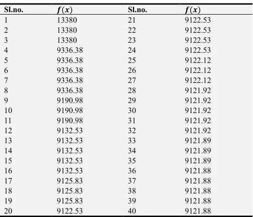
Table 1. Convergence using SA for last 40 iterations.
Sl.no. ( ) Sl.no. ( )
1 13380 21 9122.53
2 13380 22 9122.53
3 13380 23 9122.53
4 9336.38 24 9122.53
5 9336.38 25 9122.12
6 9336.38 26 9122.12
7 9336.38 27 9122.12
8 9190.98 28 9121.92
9 9190.98 29 9121.92
10 9190.98 30 9121.92
11 0.01563 31 9121.92
12 9132.53 32 9121.89
13 9132.53 33 9121.89
14 9132.53 34 9121.88
15 9132.53 35 9121.88
16 9132.53 36 9128.94
17 9125.83 37 9123.95
18 9125.83 38 9122.04
19 9125.83 39 9121.92
20 9122.53 40 9121.88
Table 2. Convergence using PA for 40 iterations.
Sl.no. ( ) Sl.no. ( )
1 13380 21 9122.53
2 13380 22 9122.53
3 13380 23 9122.53
4 9336.38 24 9122.53
5 9336.38 25 9122.12
6 9336.38 26 9122.12
7 9336.38 27 9122.12
8 9336.38 28 9121.92
9 9190.98 29 9121.92
10 9190.98 30 9121.92
11 9190.98 31 9121.92
12 9132.53 32 9121.92
13 9132.53 33 9121.89
14 9132.53 34 9121.89
15 9132.53 35 9121.89
16 9132.53 36 9121.88
17 9125.83 37 9121.88
18 9125.83 38 9121.88
19 9125.83 39 9121.88
20 9122.53 40 9121.88
The convergence has been obtained for K= 0.6 and Rw=
2.0.The minimum cost is (Rs.) 9121.88for Pattern search method in around 40 no. of iteration given in Table 2. Exactly the same values have been obtained by the method of Simulated Annealing but approximately 1000 of iterations; the last 40 value is shown in Table 1.
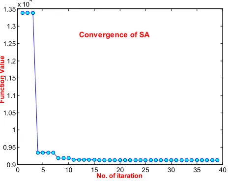
The convergence graph for Pattern Search is shown in figure 1 and for the Simulated Annealing in figure 2 respectively.
It is clear from the graph that, the search space for both the cases is almost same and convex in nature. So, there is no chance to trap in local minima.
Figure 1. Graph of the convergence for Pattern Search.
11. Conclusion
In this paper, the cost of material of a small single-phase dry transformer has been optimized using Simulated Annealing and Pattern Search Algorithm. Two design variables have been
0 5 10 15 20 25 30 35 40
0.9 0.95 1 1.05 1.1 1.15 1.2 1.25 1.3 1.35x 10
4
No. of iteration
F
u
n
ct
io
n
V
a
lu
e
chosen as the key variables viz. the e.m.f constant K and the window height/width ratio Rw .These two variables directly
affect the cost of production. CRGOS has been chosen as core material and copper as conductor material. The current density and the flux-density have been adjusted such that the design constraints are not violated and the specifications are fulfilled. The objective function (taken as the total cost of iron and copper) has been framed in terms of the design variables. The minimum cost has been found out using Simulated Annealing as well as the method of Pattern Search. Almost same answer has been obtained by Simulated Annealing with large no. of iterations; only last 40 iterations are shown in Table.1. Based on the value of the design variables found out by the program, the dimensions of the optimized transformer and the performance variables have been calculated, which is given in the Table 3. It may be noted that the design constraints have not been violated. The attempt of this paper is to establish that sometimes conventional optimization schemes like Pattern Search are capable of giving optimal solution in smaller no of steps and less computation time of 1 min 20 second compared to other complicated Stochastic Schemes of Simulated Annealing, takes 1000 of iterations and more the 2min. of time. The search space for both the cases is almost convex i.e., no. of local minima is less. So it is better before choosing the optimization Scheme, to observe the search space, no of variable and constraints, which makes the problem more complicated.
Figure 2. Graph of the convergence for Pattern.
Abbreviations
1 2
, ,
S V V Rating, KVA; Primary/ Secondary voltage, V
1, 2
I I Primary and secondary current, A
,
m
B δ Max. flux density, tesla, current density
A/sq.mm ,
s w
K K Stacking factor, window space factor , ,
w w w
H W R Window height, width, m, height/width ratio
1 2
, ,
t
E T T EMF/turn, turns of the primary and secondary
1, 2
a a Cross-section, primary and secondary in sq.mm.
Appendix A
Development of the objective function
For the given rating of transformer, EMF/turn= 5 2.236
K√ = K volts, K→e.m.f constant Maximum value of flux,
2.236 / 2
/ (4.44 ) 22 0.01007
m Et f K K
φ = = =
Net area of core,
0.01007 / 1.4 0.007
/ 36 ;
i m Bm K K
A =φ = =
Gross area of core,
0.0071946 / 0.93 0.0073
/ 6
gi i s K
A =A K = = K
For a 3-stepped core, diam. of circumscribing circle, / 0.67 0.00736 / 0.67 0.10745
gi
d = A = K = K
Window area, in m2 =
3 3
/ [2.22 .10 ] 4.692 10 /
w m w
A =S f
φ
Kδ
= x − KWindow width, in m =
/ 0.004692 / ( ) 0.0685 /
w w w w w
W = A R = KR = KR
Window height, in m = Hw =W Rw w=0.0685 Rw/K Distance between core centers,
0.10745 0.0685 /
c w w
d = +d W = K + KR
Length of the largest side of core stamping (for 3-stepped core), a=0.9d=0.0967 K
Overall width, W=dc+ =a 0.0685 / KRw +0.2042 K
Gross area of yoke is same as gross area of core assuming same flux-density in the core and the yoke.
The height of yoke, m =
/ 0.00736 / (0.0967 ) 0.08
y gi
H =A a= K K = K
Over all height, m =
2 0.0685 / 0.16
w y w
H=H + H = R K + K
Volume of iron, m3 =
2( ) 2{0.0685( / ) 0.2042 }0.0071946
i w i w w
V = H +W A = R K+ KR + K K
=0.0009856( R Kw + K R/ w) 0.002938+ K1.5
Taking density of iron as 7650 Kg/m3 and cost of high grade
CRS as Rs. 150/- per Kg. Cost of iron (Rs.), CI=
1.5
1131( R Kw + K R/ w) 3371+ K Mean length of turn, m =
( / 2) (0.10745 0.0685 / 2 / )
mt w w
L =
π
d W+ =π
K + KR0.3376 K 0.1076 / KRw
= +
Total copper area in the window, mm2
N1I1+N2= (2S.103)/ (Et. δ) =10000/ (2.236k.2.4)=1863.4/k ∴ Volume of copper =
6
1863.4(0.3376 K+0.1076 / KRw) / (K x10 )
1.5
6.292e 4 / K 2.005e 4 / (K Rw)
= − + −
Taking density of copper as 8900 Kg/m3 and the cost of
super-enameled refined copper as Rs. 450/- per Kg, the cost of copper (Rs.),CC
0 5 10 15 20 25 30 35 40
0.9 0.95 1 1.05 1.1 1.15 1.2 1.25 1.3 1.35
x 104
No. of itaration
F
u
n
c
ti
o
n
V
a
lu
e
1.5
8900 450 [6.292e 4 / K 2.005e 4 / (K Rw)]
= × × − + −
1.5
2520 / K 803 / (K Rw)
= +
The Total cost of material in Rupees (CM ) =
1.5 1.5
1131( R Kw + K R/ w) 3371+ K +2520 / K +803 / (K Rw)
Appendix B
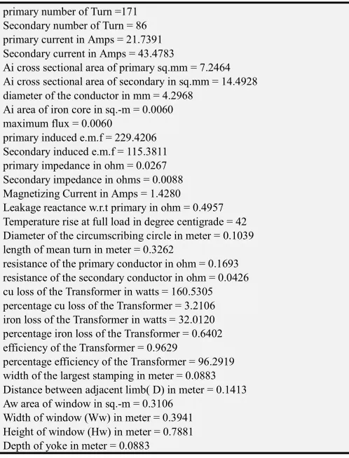
Dimensions and performance variables of the optimized transformer
The values of K & R obtained by Simulated Annealing as well as Pattern search are given below:
EMF constant, K = 0.6; Window height/width ratio, Rw= 2.
The dimensions of the optimized transformer and the corresponding performance variables are given below:
Specifications: 5 KVA, 230/115 V, 50 Hz., dry type, open (without casing).
Chosen values of other design variables:
Core material: CRGOS with stacking factor, Ks = 0.9; cost of iron/Kg = 150/-
No. of core steps = 2; Flux-density, Bm= 1 wb/m2; Iron
loss/Kg = 1.331 W
Conductor material: copper; current density = 2.4 A/mm2;
Cost of copper/Kg = Rs. 450/-
Resistivity of copper at operating temperature = 0.022 Ω/m/mm2
Table 3. Optimal Design Parameters.
primary number of Turn =171 Secondary number of Turn = 86 primary current in Amps = 21.7391 Secondary current in Amps = 43.4783
Ai cross sectional area of primary sq.mm = 7.2464 Ai cross sectional area of secondary in sq.mm = 14.4928 diameter of the conductor in mm = 4.2968
Ai area of iron core in sq.-m = 0.0060 maximum flux = 0.0060
primary induced e.m.f = 229.4206 Secondary induced e.m.f = 115.3811 primary impedance in ohm = 0.0267 Secondary impedance in ohms = 0.0088 Magnetizing Current in Amps = 1.4280 Leakage reactance w.r.t primary in ohm = 0.4957 Temperature rise at full load in degree centigrade = 42 Diameter of the circumscribing circle in meter = 0.1039 length of mean turn in meter = 0.3262
resistance of the primary conductor in ohm = 0.1693 resistance of the secondary conductor in ohm = 0.0426 cu loss of the Transformer in watts = 160.5305 percentage cu loss of the Transformer = 3.2106 iron loss of the Transformer in watts = 32.0120 percentage iron loss of the Transformer = 0.6402 efficiency of the Transformer = 0.9629
percentage efficiency of the Transformer = 96.2919 width of the largest stamping in meter = 0.0883 Distance between adjacent limb( D) in meter = 0.1413 Aw area of window in sq.-m = 0.3106
Width of window (Ww) in meter = 0.3941 Height of window (Hw) in meter = 0.7881 Depth of yoke in meter = 0.0883
Height of yoke in meter = 0.0883
Height of frame (H)frame in meter = 0.9647 Width of frame (W)frame in meter = 0.2296
References
[1] M. A. Kladas, A. G. Kladas, P. S Georgilakis, “Computer aided analysis and design of power transformers”, Science direct, Elsevier, Computers in Industry, no. 59, pp.338-350, 2008. [2] O. W. Anderson, “Optimum design of electrical machines”,
IEEE Trans., Vol.PAS-86, pp. 707-11, 1967.
[3] A. Khatri, O. P. Rahi, “Optimal design of transformer: a compressive bibliographical survey”, International Journal of Scientific Engineering and Technology, Vol. No.1, No.2, pp.159- 167, 2012.
[4] D. Mack worth, A. Poole, R. Goebel 1998, “Computational intelligence”, Oxford University Press, ISBN-0-19-510270-3. [5] J. C. Olivares-Galvan, “Selection of copper against aluminium
windings for distribution transformers,” IET Electrical Power Application, Vol. 4, no. 6, pp. 474-485, 2010.
[6] Transmission Line Data, Eastern region, West Bengal State Electricity-Transmission Co. Ltd., India, November 20-December 19, 2011.
[7] Chakraborty, and S. Halder, “Power System Analysis, Operation and Control,” New Delhi: PHI; 2010.
[8] M. Ramamoorty, ‘Computer-aided design of electrical equipment’, Affiliated East-West Press Pvt. Ltd. New Delhi, 1987.
[9] W. T. Jewell “Transformer design in the undergraduate power engineering laboratory”, IEEE Transactions on Power Systems, 1990, 5 (2), pp. 499-505.
[10] E. Rich, K. Knight 2004, “Artificial intelligence”, TMH, ISBN 0-07- 460081-8.
[11] A. K. Sawhney, “A course in electrical machine design”, Dhanpat Rai & Sons, New Delhi, 2003.
[12] M. G. Say, “Performance and design of A. C. Machines”, ELBS.
[13] A. Shanmugasundara, G. Gangadharan, R. Palani, “Electrical machine design data book”, Wiley Eastern Ltd.1979.
[14] A. E. Dymkov, “Transformer design, MIR publications”, 1975. [15] H. M. Rai, “Principles of electrical machine design”, Satya
Prakashan, New Delhi, 1985.
[16] S. S. Rao, “Engineering Optimization–Theory and Practice, Third Edition”, New Age International (P) Ltd., 1996. [17] K. Deb, “Optimization for engineering design”, PHI, 2010. [18] N. S. Kambo, “Mathematical programming techniques”,