The effect of irrigation practice on drainage and solute leaching under spray irrigation on a stony soil

(1)

Lincoln

University

Digital

Dissertation

Copyright

Statement

The

digital

copy

of

this

dissertation

is

protected

by

the

Copyright

Act

1994

(New

Zealand).

This

dissertation

may

be

consulted

by

you,

provided

you

comply

with

the

provisions

of

the

Act

and

the

following

conditions

of

use:



_you

_will

_use

_the

_copy

_only

_for

_the

_purposes

_of

_research

_or

_private

_study



you

will

recognise

the

author's

right

to

be

identified

as

the

author

of

the

dissertation

and

due

acknowledgement

will

be

made

to

the

author

where

appropriate



you

will

obtain

the

author's

permission

before

publishing

any

material

from

the

(2)

The Effect of Irrigation Practice on Drainage and Solute Leaching

Under Spray Irrigation on a

Stony Soil

A Dissertation

submitted in partial fulfilment

of the requirements for the Degree of

Bachelor of Science with Honours

at

Lincoln University

by

Balin Burns Robertson

Lincoln University

(3)

Abstract of a Dissertation submitted in partial fulfilment of the

requirements for the Degree of Bachelor of Science with Honours.

Abstract

The Effect of Irrigation Practice on Drainage and Solute Leaching

Under Spray Irrigation on a

Stony Soil

by

Balin Burns Robertson

Research was conducted to assist in the improvement of irrigation efficiency on the shallow stony soils

of Canterbury and identify the effect of current irrigation practice on the redistribution of solute within

the soil profile. Irrigation treatments were measured using twenty-four undisturbed monolith

lysimeters containing a stony Eyre shallow silt loam soil. Treatments included 15/10, 15/15, 30/20,

30/30, 60/40 and 60/60, being the respective soil deficit irrigation trigger/irrigation depth

combinations (mm). The trial was split into three experiments. Experiment 1 began with a surface

application of bromide tracer before exposing the lysimeters to the irrigation treatments for three

months. Experiment 2 and 3 were designed to examine how the bromide had been redistributed within

the pores during Experiment 1. Experiment 2 irrigated 250 mm depth continuously at 50 mm/hr to

drain bromide in the macropores, while Experiment 3 irrigated 500 mm depth continuously at 2 mm/hr

to drain bromide in the soil matrix. Over the three experiments, leachate was collected regularly and

analysed for bromide.

Preferential flow dominated solute leaching, occurring in the first drainage event irrespective of the

application volume and frequency of irrigation, with leached bromide moving predominately through

the macropore fraction of the soil. Treatments with greater irrigation quantities corresponded with

more extensive preferential flow, drainage and for the most part, leaching in Experiment 1. Treatments

irrigated to field capacity (FC) had greater leaching and drainage as well, as uniform irrigation of

lysimeters in a treatment meant soil heterogeneity caused some lysimeters to exceed FC before others.

Generally, there were no significant treatment effects on the cumulative bromide leached across the

experiments, reflecting the dominance of preferential flow under the irrigation conditions studied.

There was evidence that bromide distribution in the profile at the end of Experiment 1 was affected

(4)

readings in Experiment 2, while the moisture deficit irrigation trigger influenced the bromide peak

mass and cumulative mass readings in Experiment 3. However, effects were not consistent across

treatments and experiments, making interpretations difficult.

The results indicate that irrigation practices on Eyre shallow silt loam soils at 50 mm/hr needs to be

adjusted for preferential flow, which has a dominant influence on solute distribution within the soil

profile. Results imply that the 15/10 treatment had the least leaching as less extensive preferential

flow means solute remains within the profile and has a greater opportunity to be immobilised.

(5)

Acknowledgements

This year has been one of the most intense times of my life, and I am grateful to the following people

for their support and assistance, without which I would not have hoped to have completed this project.

Foremost, Dr Sam Carrick for the countless hours of your time that you dedicated into guiding me

through my honours year. It was an absolute privilege to have you as a supervisor and know that I will

be forever grateful for your help and guidance.

The team at Plant and Food Research, Steve Thomas, Gina van der Klei, Frank Tabley, Trish Fraser, Chris

Dunlop and Rogerio Cichota, your patience in dealing with my constant pestering is amazing and I have

learned a great deal due to your support and can’t thank you enough for your ongoing assistance and

involvement throughout the project. Cheers for the lysimeters as well.

To my family for their tremendous amount of support and encouragement.

And a special thanks to Veronica Penny, who has kept me company on many a light night working at

(6)

List of Tables

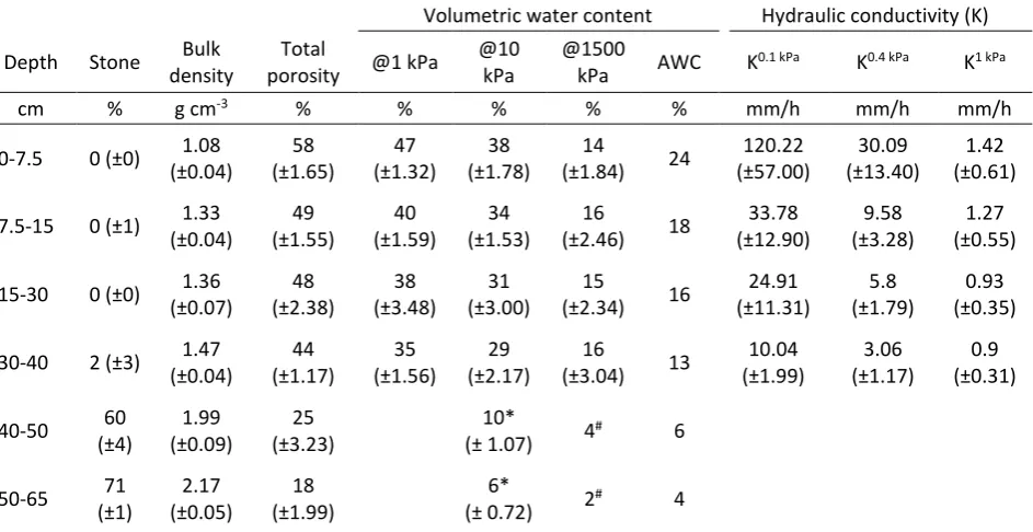
Table 1 Irrigation treatments and associated moisture status. ...17 Table 2 Average hydraulic soil properties. Values in brackets were the calculated standard

deviation. Soil properties to the depth of 40 cm were measured from 10x7.5 cm soil cores using pressure plate and tension table apparatus (Carrick, 2009). Soil properties below 40 cm were measured in the field using the volume replacement method (Hedley et al., 2012). ...21 Table 3 Experiment 1 irrigation applied and drainage for the different treatments. Drainage values

(9)

List of Figures

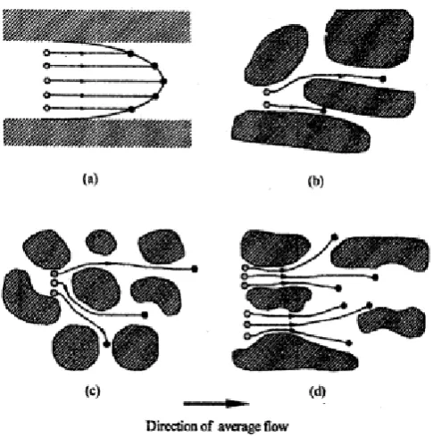
Figure 1 Schematic concepts contributing to mechanical dispersion; a) pore wall frictional drag, b) pore size effect on mean solute velocity, c) pore tortuosity, d) solute

convergence/divergence (Leij & Van Genuchten, 2001). ... 5 Figure 2 Descriptive diagram of the dispersal of a band of solute during convective transport

through a soil (Carey, 1993). ... 6 Figure 3 Lysimeter TDR distribution. ...15 Figure 4 Experiment 1, wetting and drying cycles for deficit-irrigated treatments. Top graph: 15/10 treatment; middle graph: 30/20 treatment; bottom graph: 60/40 treatment. ...23 Figure 5 Experiment 1 wetting and drying cycles for the field capacity-irrigated treatments. Top

graph: 15/15; middle graph: 30/30; bottom graph (60/60). ...24 Figure 6 Experiment 2 cumulative drainage. Number labels refer to the lysimeter where drainage

results were collected from. ...25 Figure 7 Experiment 3 cumulative drainage. Number labels refer to the lysimeter where drainage

results were collected from. ...26 Figure 8 Bromide concentration breakthrough for deficit-irrigated treatments during Experiment 1

(left graph), Experiment 2 (centre graph) and Experiment 3 (right graph). C is the concentration of bromide in the soil leachate. C0 is the concentration of the bromide solution that was initially applied to soil. Treatments shown are 15/10 (Top graphs); 30/20 (middle graphs); 60/40 (bottom graphs). ...28 Figure 9 Bromide concentration breakthrough for field capacity-irrigated treatments during

Experiment 1 (left graph), Experiment 2 (centre graph) and Experiment 3 (right graph). C is the concentration of bromide in the soil leachate. C0 is the concentration of the bromide solution that was initially applied to soil. Treatments shown are 15/15 (Top graphs); 30/30 (middle graphs); 60/60 (bottom graphs). ...29 Figure 10 Treatment average peak concentrations for Experiment 3. C is the concentration of

bromide in the soil leachate. C0 is the concentration of the bromide solution that was initially applied to soil. Vertical bars represent standard error of the mean. ...31 Figure 11 Bromide mass breakthrough for deficit-irrigated treatments during Experiment 1 (left

graph), Experiment 2 (centre graph) and Experiment 3 (right graph). Treatments shown are 15/10 (Top graphs); 30/20 (middle graphs); 60/40 (bottom graphs) ...33 Figure 12 Bromide mass breakthrough for field capacity-irrigated treatments during Experiment 1

(left graph), Experiment 2 (centre graph) and Experiment 3 (right graph). Treatments shown are 15/15 (Top graphs); 30/30 (middle graphs); 60/60 (bottom graphs). ...34 Figure 13 Treatment average peak mass readings for Experiment 2. Vertical bars represent

standard error of the mean. ...36 Figure 14 Treatment average cumulative mass bromide for standardised drainage in Experiment

3. Vertical bars represent standard error of the mean. ...37 Figure 15 Treatment average peak mass readings for Experiment 3. Vertical bars represent

standard error of the mean. ...38 Figure 16 Treatment average, cumulative dry matter yield for three pasture cuts (20/4/16;

15/6/16 and 12/7/16). Vertical bars represent standard error of the mean. ...39 Figure 17 Treatment average, cumulative bromide uptake for three pasture cuts (20/4/16;

(10)

Chapter 1 Introduction

The area of irrigated land in New Zealand is rapidly increasing, being strongly linked to intensive land

use, in particular dairy farming. It is well established that irrigation can have significant benefits to

agriculture, increasing plant yield and allowing previously unproductive land to be of economic benefit.

However, current environmental research has shown these practices can have detrimental effects, by

promoting solute transport and the leaching of nutrients like nitrate (Di & Cameron, 2002b; Heckrath

et al., 1995). In light of this issue, it is necessary to understand how irrigation affects solute leaching

and hence how specific management practices may enhance or mitigate leaching losses.

In recent years, the risk of enhanced solute transport in the Canterbury region has increased over

significant areas, considering the region represents approximately 60% of New Zealand’s irrigated land

area, with recent land conversions to dairy (and irrigation) situated predominately on stony soils

(Cichota et al., 2016). Such soils are characterised by low water holding capacity, and considered

vulnerable to nutrient leaching losses and preferential flow (Carrick et al., 2013). Current literature has

predicted that the adoption of irrigation on these soils will induce nutrient leaching, especially under

poor irrigation practice and high application rates (Carrick et al., 2014; Di & Cameron, 2002a). However,

the actual dynamics of solutes within these soils under different irrigation regimes is poorly

understood or quantified, especially the effects of soil antecedent conditions, irrigation rate and

irrigation frequency (Cichota et al., 2016; Lilburne et al., 2010).

Quantification of these processes has become of increasing importance in New Zealand, especially

with the implementation of the National Policy Statement for Freshwater Management (NPS-FM) in

2011. Growing public demands for sustainability, and a necessity to maintain the country’s ‘clean

green’ image, made it necessary to develop enforceable limits of water quality and quantity. Under

the NPS-FM, regional councils are required to develop regional plans that detail rules on land and water

use as directed by national bottom lines and compulsory water values (Ministry for the Environment,

2014). In Canterbury, this is seen in the form of the Land and Water Regional Plan (LRWP), which

specifies maximum annual amounts of nutrients (such as nitrate) that can be lost from a system

(Environment Canterbury, 2015). In light of this, it is necessary to determine best management

strategies for irrigation that can be used to minimise leaching, so farms don’t exceed nutrient caps.

However, current research on solute dynamics under irrigation has not caught up to policy or

(11)

1.1 Aim and objectives of the study

The main aim of the project is as follows:

 To assist in the improvement of irrigation efficiency on the shallow stony soils of Canterbury

and identify the effect of current irrigation practice on the redistribution of solute within the

soil profile.

To achieve this goal, the main objectives of the study were as follows:

 To quantify different drainage and solute losses under varying irrigation return intervals.

 To quantify different drainage and solute losses that occur when soils are irrigated to field

capacity or a determined moisture deficit.

 To quantify the redistribution of solute in the soil profile with variation in irrigation practice.

The hypotheses of the project were as follows:

 Irrigation to refill a greater soil moisture deficit will increase the rate of drainage and solute

leaching.

(12)

Chapter 2 Literature Review

2.1 Quantifying drainage and solute transport behaviour

Quantification of soil drainage and solute leaching is a notoriously difficult task. Undisturbed soil can

cause issues due to the inherent soil heterogeneity, while factors such as measurement scale and

labour restraints cause some methods to become unsuitable. Of the many methods that have been

developed, lysimeters have been found to be highly versatile and accurate for free draining soils.

Capable of using both repacked and undisturbed soil, lysimeters can be engineered to specific

measurement requirements or be used to reproduce soil field conditions. Lysimeters also have a

significant advantage to field studies, whereby it is possible to collect lysimeters from different

locations and transport them back to a research facility, where it is possible to better control variables

such as rainfall or irrigation.

As with any method, lysimeters have their restrictions. Repacked lysimeters have been criticised for

the alteration of water flow paths and the formation of artificial soil systems (Cassel et al., 1974). This

has caused significant over estimation of drainage and nitrogen flux, with a study by Pakrou and Dillon

(2000) over estimating drainage in an irrigated paddock by 78%. The use of undisturbed monolith

lysimeters allows a more natural quantification of solute and water flux. However, issues have been

raised with collection techniques as a result of soil compaction due to friction between the soil and the

walls of the lysimeter (Klocke et al., 1993). Developments in lysimeter extraction, with a focus on

supporting soil pedestals has meant monolith lysimeters can be collected without alteration of physical

properties (Bowman et al., 1994). While the application of liquefied petrolatum can fill the gap

between the monolith and lysimeter casing, preventing preferential edge flow (Cameron et al., 1992).

However, considering a limited volume of soil is removed from the field, it must be determined

whether the volume measured is representative of the variability of the studied soil or parameter.

Multiple studies have demonstrated that significant soil heterogeneity can exist within small areas of

land (Hbirkou, 2011; Hillel, 1998), with even small variations in soil properties resulting in significant

differences in the leaching characteristics of a soil (Lilburne & Webb, 2002). As a result, soil physics

research studies need to take into account the potential effect of the representative elementary

volume (REV), which is the smallest volume required to represent the variation in element forms and

proportions within a given system (Bear, 1972). The size of the REV varies spatially and depends on the

(13)

& Papadopoulos, 2010; Richard & Steenhuis, 1988). Li et al. (2009), found for a cracked clay soil, an

REV of width 0.29 m could be used for determining water movement. While Lauren et al. (1988)

estimated an REV with a representative area of 0.5 m2_{is necessary. These studies demonstrate that a}

lysimeter with conventional dimensions (50 cm width by 70 cm depth, and 0.2 m2 _{area) may have issues}

in capturing the REV for leaching studies through soils that have significant macropore flow. As a result,

this may be a source of variation in the leaching behaviour between replicate lysimeters in a trial, and

needs to be considered when interpreting trial results.

2.2 Modes of water flow and solute transport through soil

When soil moisture content exceeds field capacity (FC) (-5 to -20 kPa suction, depending on soil

physical properties), the soil is unable to store water, causing water to drain through the profile.

Solutes in the soil solution (such as bromide and nitrate) can be mobile, and are therefore leached

when drainage occurs (Malcolm, 2013). Due to this, the movement of water significantly affects how

solutes are transported through the soil. When there is negligible water movement, diffusion is the

governing mechanism of solute transport. As water movement becomes more significant, solutes

move in relation to convective and hydrodynamic dispersion (matrix flow) or preferential flow.

2.2.1 Diffusion

Diffusion is the dominant spreading mechanism under low flow rates or for short travel distances (Flury

& Gimmi, 2002). Its importance in solute investigations is generally negligible, as project conditions are

commonly saturated or continuous unsaturated flow. However, in investigations involving intermittent

water application such as irrigation, with periods of no drainage and soil drying by evapotranspiration

and low water flux, diffusion can have a significant effect on solute movement (Gerke & Kohne, 2004).

The underlying method of transport occurs as a result of Brownian motion, where repeated deflections

and collisions of molecules in fluid cause solutes to equalise in terms of spatial distribution (Hillel,

2003). Therefore, solutes move in response to a concentration gradient and can be described by Fick’s

Law:

𝐽_𝑑= −𝐷_𝑠𝑑𝑐_𝑑𝑥 (1)

where Jd is the rate of diffusion, Ds is the diffusion coefficient of the solute in soil as determined by soil

moisture content and dc/dx is the solute concentration gradient (McLaren & Cameron, 1996).

2.2.2 Matrix flow

As water flux increases, the mechanisms of convection and hydrodynamic dispersion dominate solute

(14)

occurs with a mass flow of water through soil (Hillel, 2003). Darcy’s Law, with an additional solute

concentration function c, describes this transport (Hillel, 2003):

𝐽𝑐 = 𝑞𝑐 = −𝑐(𝑘𝑑𝐻_𝑑𝑥) (2)

where Jc is the convective solute flux, c is the solute concentration, q is water flux, K is the hydraulic

conductivity and dH/dx is the hydraulic gradient (McLaren & Cameron, 1996). By this mechanism

alone, a band of solute would move as a single wetting front, as dictated by the average pore velocity

(McLaren & Cameron, 1996). However, due to soil heterogeneity, solute breakthrough undergoes

mechanical mixing known as hydrodynamic dispersion. This mixing is a function of the varying pore

sizes, lengths and tortuosity found within a soil (Figure 1). Some solute moves rapidly through large

pores, while other solute moves slower through smaller pores (Dennis, 2009). Even within a pore,

solute is prone to a velocity gradient due to frictional drag between the pore wall and moving soil

water (Carey, 1993). Pore pathways may also be tortuous, with some pathways being longer than

others to cover the same distance down the soil (Dennis, 2009). As a result, some solute tends to drain

faster and/or slower than other solute, causing solute breakthrough to become dispersed, even with

a uniform wetting front (Figure 2).

(15)

Figure 2 Descriptive diagram of the dispersal of a band of solute during convective transport through a soil (Carey, 1993).

2.2.3 Preferential flow

Preferential flow is defined as “all phenomena where water and solutes move along certain pathways,

while bypassing other volume fractions of the porous soil matrix” (Gerke, 2006). These phenomena

result in a spatially irregular wetting of the soil profile, as water moves faster and with higher quantity

at certain locations of the soil (Šimůnek et al., 2003). These flows commonly develop into “finger”-like

flow patterns, representing the channels of concentrated water flow through the soil (Rezanezhad et

al., 2006). Quantification of this phenomenon is difficult as it is affected by many factors and can exist

in multiple forms. In general, preferential flow is classified in to three differing categories: macropore

flow, unstable flow and funnel flow (Gerke, 2006).

Macropore flow

Macropore flow is described as rapid non-equilibrium channel flow through structural pores in the soil

(Šimůnek et al., 2003). The definition of macropore flow is flexible, with flow paths varying from

individual pores of different size to highly connected pore networks (Gerke, 2006). The significance of

preferential flow to solute leaching can vary depending on macropore continuity, tortuosity and

density (Jarvis, 2007). Macropores with the greatest leaching potential are generally surface connected

and have a low tortuosity in the case of sorbed solutes (Allaire et al., 2002). These pores become active

in response to a prevailing pressure potential gradient (Jarvis, 2007). When the application of water

exceeds the rate with which the finer pore fraction of the soil can conduct, water moves into larger

pores as the water entry potential of macropores is exceeded (Hendrickx & Flury, 2001). A wide range

(16)

plant roots or earthworms, cracks produced by shrinkage of clay soils, chemical weathering of bedrock

material, freeze-thaw cycles and soil cultivation (Beven & Germann, 1982). The presence of rock

fragments has also been shown to influence macropore flow, causing an increase in the mean radius

of macropores (Shi et al., 2012), producing voids along soil-stone interfaces in shrinking-swelling soils

(Sauer & Logsdon, 2002) and influencing the direction of root growth (Schwärzel et al., 2012).

Unstable flow

Unstable flow generally occurs in the matrix of coarse textured soils as a result of instabilities in the

waterfront (Larsson et al., 1999). Instabilities develop from perturbations in the wetting front caused

when the matric potential behind the front opposes the flow (Wang et al., 2003). The mechanism for

water front perturbation can vary between soils and includes air pressure build-up ahead of the

wetting front (Hill & Parlange, 1972), water repellency (Wang et al., 2000) and at fine-over-coarse

textural layers (Dobrovolskaya et al., 2014). As a result of water front perturbation, wetting fronts are

refined to small areas of infiltration. Redistribution of water creates a matric potential reversal, causing

flow to move preferentially through these infiltrating areas to form ‘fingers’ of rapid water flow (Wang

et al., 2003).

Funnel flow

Funnel flow refers to situations where parts of the soil behave like the wall of a funnel, deflecting

unsaturated flow into spatially concentrated columns of rapid water movement (Nimmo, 2005). The

concentration of water corresponds with an increase in hydraulic conductivity and is commonly

associated with contrasting soil layers or lenses (Kung, 1990b). In a lab study, Kung (1993) found that

funnel flow would occur along an inclined boundary when there is a macroscopic Haines jump (a

high-speed pore scale event (Armstrong et al., 2015)) across the boundary and water application rates were

smaller than a certain critical rate.

The effect of these phenomena on solute transport can vary. Many studies observe preferential flow

causing rapid movement of solute through the soil profile leading to enhanced solute leaching

(Blackwell, 2000; Reichenberger et al., 2002; Tyner et al., 2007). Alternatively, a few studies have

observed solute leaching had reduced as a result of preferential flow (Cote et al., 2000; Dennis, 2009;

Larsson & Jarvis, 1999). From these studies, solute placement appears to govern whether preferential

leaching or preferential bypass occurs (Dennis, 2009). If the solute is located near macropores it will

be prone to leaching, while solute found in the less permeable region of the soil matrix is protected

(17)

2.3 Importance of preferential flow to sustainable land management

The importance of preferential flow has increased over time as old perceptions of soil homogeny and

solute transport by matrix flow has changed. Reliance on lab studies developed a perception of a strong

interaction of drainage with the soil matrix, and hence many solutes were thought to have negligible

leaching due to soil sorption (Flury, 1996). However, increasingly studies have found preferential flow

can significantly affect solute losses and land management (Anyusheva et al., 2016). Everts and

Kanwar (1990) observed preferential flow transported as much as 24% of the bromide and 20% of the

nitrate that leached into a subsurface drain, while contributing to only 2% of the total drainage.

Shipitalo et al. (1990) found similar results, with a small fraction of the soil accounting for 70% of the

total leaching from a 60 mm water application.

Even pesticides, thought to be strongly sorbed to the soil and of low leaching susceptibility have been

lost from systems in significant quantities due to preferential flow (Flury, 1996). Wettstein et al. (2016)

found rapid breakthrough of thiamethoxam, and three other highly sorbed pesticides even though the

first drainage event didn’t occur until 15 days after application. While Flury et al. (1995) found that

three pesticides with varying sorption strengths moved to the same maximum depth due to

preferential flow. Although preferential flow may only equate to small annual pesticide loss rates,

which can range from 0.1% to several percent (Flury, 1996; Wettstein et al., 2016), even small

proportions of leached pesticide can have significant effects on ecosystem or human health (Klaus et

al., 2014).

It can be gathered from the literature that when preferential flow is present, it can account for

substantial leaching losses from a soil. The frequency with which it occurs is in some debate however,

due to the highly variable nature of the phenomena. Graham and Lin (2011) found in 175 rainfall

events, preferential flow occurred at 17 to 54% of the events at each of the 10 sites monitored in the

study. However, when viewed holistically, preferential flow occurred in at least one site during 90% of

the rainfall events (Graham & Lin, 2011). Wiekenkamp et al. (2016) had similar results in a catchment

scale study, with preferential flow occurring in 7 to 51% of the measured rainfall events. It was found

that preferential flow could be highly uniform during large storm events (>25 mm), but was otherwise

governed by small scale soil and biological features (Wiekenkamp et al., 2016). This indicates the

difficulty in developing management practices to reduce forms of preferential flow, as the phenomena

are variable over space and time, with the parameters governing preferential flow still understudied.

2.3.1 Studies of preferential flow in New Zealand soils

In New Zealand, studies have been aimed at identifying soils susceptible to preferential flow. A few

(18)

soils (Aislabie et al., 2001; Pang et al., 2008). This was generally attributed to the soils having a fine

uniform soil structure that kept the soils well-drained and minimised preferential flow (Aislabie et al.,

2001). However, even these soils could demonstrate preferential flow under the right conditions with

multiple studies demonstrating the development of funnel flow in volcanic soils as a result of

hydrophobicity (Barkle et al., 2014; Muller et al., 2010). Well-drained silt loam soils, such as Waikiwi

and Templeton silt loams demonstrated higher susceptibility to preferential flow, however soils that

were poorly drained or stony are found to be the most susceptible (McLeod et al., 2003; McLeod et

al., 1998; Pang et al., 2008). Poorly drained soils such as Gley soils are generally associated with

cracking and a soil matrix of low hydraulic conductivity, causing water and solute to move

preferentially down macropores (Li et al., 2009). For stony soils, susceptibility to preferential flow is

commonly attributed to a low water holding capacity and a moderate to rapid permeability (Carrick et

al., 2014). However, solute dynamics in these soils is understudied. Most research is confined to

constant saturated or unsaturated conditions (Cichota et al., 2016; Pang et al., 2008), which indicate

strong preferential flow, however may be biased due to unnatural wetting conditions. Transient

condition studies have more variable results. Carrick et al. (2014) observed preferential flow in a

Selwyn stony soil in a periodic irrigation experiment even though the trial followed best management

practices in terms of irrigation rate (35-40 mm/hr) and application volume (12-18 mm). In contrast,

Close et al. (2010) on a Lismore stony soil, found low faecal coliform leaching under a travel irrigator

which applied 55 mm of irrigation. However, when irrigation application increased to 80 mm, leaching

became more apparent (Close et al., 2010). Thus, stony soils may be susceptible under some

conditions, but can have negligible preferential flow in others. This demonstrates an important area of

research to be studied, as no papers can be found that have done systematic trials on stony soils, to

see how solute transport is affected by different irrigation practices and antecedent soil moisture

conditions. As a result, the effectiveness of current irrigation practices can only be assumed, with little

research to be found for an informed judgement.

2.4 Effect of irrigation practices on solute transport

2.4.1 Introduction

Irrigation is now an intrinsic part of agriculture in New Zealand and generally signifies an increase in

productivity and land-use intensification. The method of application can vary but is progressively

becoming dominated by spray systems in the form of centre pivots (Statistics New Zealand, 2012).

Older methods of flood irrigation are being replaced over time by centre pivots due to the need for

greater water-use efficiency and nutrient management (Cichota et al., 2016). Centre-pivot systems are

(19)

solute leaching from a soil is still uncertain however, as patterns in water movement can vary

significantly with differing soils, boundary conditions and plant cover.

2.4.2 Initial soil water content

The initial saturation of the soil prior to irrigation can significantly influence the hydrological properties

of the soil. At high initial water saturation, pulses of solute tend to bypass a greater proportion of the

smaller pores, which when filled with water have low conductivity (Hamlen & Kachanoski, 2004). As a

result, water and solute tend to flow preferentially down macropores with high conductivity (Lewan

et al., 2009; Schaetzl & Thompson, 2015; Vereecken, 2005). Quisenberry and Phillips (1976) observed

this, with 20% of a 42 mm water application penetrating below the 90 cm depth immediately after

application, even though initial soil moisture was below FC.

Alternatively, dry soil conditions can cause preferential flow due to the presence of hydrophobicity

and soil cracking (Barkle et al., 2014; Bronswijk, 1991; Ritsema et al., 1998). Ritsema et al. (1998)

identified the formation of a non-uniform wetting front in a dry soil due to lateral transport of water.

This occurred under extreme conditions, as the dry soil was water repellent, resulting in wetting fronts

infiltrating deeper in areas of the soil with higher antecedent water content. It has also been found

that drier soils may enhance preferential flow by reducing the lateral losses from preferential flow

paths (Jarvis, 2007). Multiple studies have demonstrated initially dry soils as having more rapid and

significant preferential flow to soils of higher water content (Babel et al., 1995; Merdun et al., 2008;

Shipitalo & Edwards, 1996). However, the requirement of dry soils (c. 11% water content; [Merdun et

al., 2008; Shipitalo & Edwards, 1996]) may mean preferential flow maybe less likely to arise from this

phenomena in irrigated pasture. However, Kung et al. (2006) had variable results, as application of

bromide to dry soil caused leaching to reduce. It was speculated that the dry surface conditions would

result in many small pores near the soil surface with negative matric potentials. This would cause

bromide to infiltrate into the small pore fraction, causing bromide to be less susceptible to macropore

flow (Kung et al., 2006).

2.4.3 Influence of Irrigation rate and volume

The quantity and intensity of irrigation can strongly affect water and solute transport. High irrigation

volumes generally correspond with a greater leaching depth; however, results vary pending on

irrigation rate (Yang, 2014). If the rate is lower than the maximum infiltration rate of the soil matrix,

water flow occurs predominately by uniform matrix flow (Schaetzl & Thompson, 2015). As a result,

draining water only reaches a depth relative to the volume of infiltrating water. When irrigation rate

exceeds the infiltration capacity of the soil matrix, water tends to flow through macropores forming

(20)

(Dennis, 2009). On a stony Lismore soil, Cichota et al. (2016) was able to observe this relationship, with

preferential solute transport seen to be greater at 20 mm/hr compared to 5 mm/hr. Gray et al. (2016)

found a similar effect in a transient moisture study on an Eyre shallow silt loam, with increased

cumulative drainage when irrigation rate increased from 12 to 50 mm/hr irrigation. However, the rate

effect on phosphorus leaching was marginal, and indicates that irrigation rate may not be a dominant

influence on leaching in the studied stony soil (Gray et al., 2016).

If irrigation is of a great enough volume, preferential flow can also be induced as infiltration rates

decline with the filling up of soil pores, causing water to preferentially move down macropores (Kohne

& Gerke, 2005; Kung et al., 2006; Schaetzl & Thompson, 2015). Kohne and Gerke (2005) observed this,

with a rate of only 7 mm/hr causing preferential flow in a tile drained field soil. Non-uniform wetting

fronts can also be developed as a result of water ponding and micro topography. Cook (1983) observed

high rate irrigation could facilitate the preferential infiltration of water at micro-topographical

depressions on the soil surface. Clothier and Heiler (1983) had similar results, however rate did not

appear to be a major influence, with a significantly higher fraction of water infiltrating at the low points

in the micro-relief at rates as low as 4.1 mm/hr.

2.4.4 Irrigation timing

Irrigation timing has complicated effects on drainage and solute movement. Firstly it affects the initial

water content of the soil prior to irrigation, influencing properties such as infiltration and matric

potential. Frequent irrigation is likely to result in a soil with a relatively high water content, while the

longer the between irrigation period, the greater the opportunity for hydrophobicity and soil cracking

to occur (the effect of which is described in section 2.4.2 Initial soil water content).

Secondly, it affects the dynamics of solute and water. Under saturated flow, the hydraulic head or

gravitational potential is the primary driver of the downward flow of water (Nimmo, 2005).

Alternatively, in unsaturated conditions, water movement is driven by differences in water potential

(Nimmo, 2005). This causes water to move in variable directions, which can be lateral, downward, or

even upward in response to evaporation (Schaetzl & Thompson, 2015). The effect of this is a

redistribution of solute in the soil profile, which can have variable effects on solute leaching. Some

studies have seen a significant increase in solute leaching as a result of transient soil moisture

conditions (Lewan et al., 2009; Meyer-Windel et al., 1999). Cote et al. (1999); (2000) found that flow

interruptions and the development of transient conditions caused bromide leaching to increase by

10-20% compared to continuous flow leaching. Alternatively, other studies have found transient

(21)

Effects seem to depend on the severity of the transient conditions. At short intervals, interruption in

flow allows solute to diffuse from less permeable regions of the soil matrix to the boundary of

preferential flow paths. As a result, solute is prone to leaching with a continuation in water flow. This

can lead to the enhanced leaching found by Cote et al. (2000), however, if preferential flow does not

occur (matrix flow instead), a reduction in leaching occurs (Meyer-Windel et al., 1999).

Under more severe transient conditions, the process of drying causes the redistribution of bromide

from larger pores to smaller pores. Sambale et al. (2000) observed bromide under very dry conditions,

moving from macropores into the finer pore fraction. In these smaller pores, pore water velocity was

low, thus reducing the amount of leaching. However, over multiple wetting events, bromide

remobilised and was again susceptible to leaching (Sambale et al., 2000).

The limitation with current literature is that studies have focused on the extremities of antecedent

conditions. As such, the ‘antecedent conditions’ that have been researched are either developed over

the soil draining from saturated flow to FC (Cote et al., 2000), or over months without water (Sambale

et al., 2000). As a result, the redistribution of solute that would occur under conventional irrigation

practice is still relatively unknown.

2.5 Research gaps and the importance of the current study

It was detailed in the Introduction that there is a practical demand for transient irrigation studies to

determine practices with the lowest leaching risk, as required by new legislation on water

management. In Canterbury, studies on stony soils are of significant interest, as they dominate the

irrigated land area in the region and are still relatively understudied in terms of solute and drainage

dynamics. From the literature, preferential flow appears to be a major contributor to the mobility of

solute within a soil, with the proportion of the active pore volume in this phenomenon being small

relative to the quantity of leaching it can cause. However, it has been shown that preferential flow can

be initiated by a number of mechanisms and have varying effects on leaching depending on a number

of conditions such as soil type, initial soil moisture content, application volume, application rate and

strength of antecedent conditions. Limitations in research surrounding the effect of these factors in

relation to the transient moisture conditions expected under ‘real’ irrigation practice, means there is

a deficit in knowledge to back up best management practices for reducing leaching from irrigation.

This dissertation aims to assist in the improvement of irrigation efficiency on shallow stony soils by

researching the following knowledge gaps:

 There is little experimental research on how solute is redistributed within the soil as a result

of transient conditions caused by irrigation. This could have significant implications to the

(22)

in and hence its susceptibility to different forms of water movement. Two drainage events are

used in this study to explore the effect of different irrigation practices on the locality of solute

in the soil profile.

 Stony soils have been classed as susceptible to preferential flow and solute leaching. However,

the conditions that govern the initiation or extent of this phenomenon in these soils are not

well understood. Using different irrigation practices, this study explores how preferential flow

maybe influenced by variation in application volume, antecedent conditions and the moisture

(23)

Chapter 3 Materials and Methods

3.1 Soil description

Solute leaching measurements were made on 24 undisturbed soil monolith lysimeters. Lysimeters (50

cm diameter by 65 cm depth) were collected during a previous 2013 project from an irrigated sheep

grazed pasture at the AgResearch Research Farm, Canterbury (43.62 °S, 172.47 °E). The soil was a

free-draining Eyre shallow silt loam (Orthic Recent soil [Hewitt, 2010]) with four distinct layers, including a

stoneless topsoil and B-horizon overlying two very stony horizons, one with a silt loam matrix and the

other a sand matrix (Appendix A). Soil physical properties are described in Table 2 (Section 4.1 Soil

properties), based on soil samples collected in undisturbed soil adjacent to the lysimeter collection pit.

For the stone free layers (0 – 40 cm depth) undisturbed soil cores (10 cm diameter x 7.5 cm depth)

were hand carved from each depth increment to measure soil bulk density, porosity, water release

and hydraulic conductivity at the Landcare Research soil physics lab. In the stony horizons it is not

possible to collect soil cores, so a volume replacement method (Hedley et al., 2012) was used to

calculate stone content, bulk density and porosity. Water holding porosity and unsaturated

conductivity were not measured on the gravelly horizons.

Based on this measured data, an average pore volume (PV) was estimated at approximately 249 mm

for the soil volume within the lysimeters. Total porosity averaged 50% in the top 40 cm (fine earth

fraction) while stone content reached 71% at the base of the lysimeters, reducing the porosity of the

gravel layers down to 18-25%.

3.2 Lysimeter installation

Collection of lysimeters followed the procedure given in Cameron et al. (1992). This involved working

a metal cylinder casing (50 cm diameter by 70 cm depth) into the soil while carefully digging around

the casing to minimise disturbance of soil structure, and leaving an undisturbed soil monolith with an

actual soil column length of 65 cm within the casing. To prevent preferential edge flow down the casing

wall, lysimeters were sealed using petroleum jelly. The lysimeters are then separated from the

underlying gravels using a hydraulic ram to insert a cutting plate at the bottom of the lysimeter.

Following this, the cutting plate is replaced with a drainage base that collects lysimeter drainage

through a centre drainage hole.

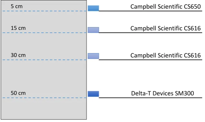
Plastic tubing connected to the base of each lysimeter directed any drainage or solute to a tipping

(24)

Figure 3), which were used to determine the soil water deficit for each lysimeter, and consequently

the timing of irrigation. A CR1000 Campbell Scientific data logger recorded soil moisture sensors and

tipping spoon drainage data at 10-minute intervals.

Figure 3 Lysimeter TDR distribution.

Herbage on the lysimeters was a mixed sward dominated by rye grass, and was allowed to grow to

enhance soil moisture loss through evapotranspiration. Herbage growth rate was maintained by

applying 250 kg/ha of superphosphate and 100 kg/ha urea prior to the start of the experiment

(22/12/15), and 50 kg N/ha as calcium ammonium nitrate fertiliser on the 15th_{April 2016, to ensure}

herbage growth was not nutrient limited during the experiment. Lysimeters were located at the Plant

and Food Research lysimeters facility at Lincoln, which included a rain out shelter (Plate 1). The rain

out shelter was a cover that automatically moved over the lysimeters during rain, but otherwise left

lysimeters exposed to climatic conditions.

Campbell Scientific CS650

Campbell Scientific CS616

Delta-T Devices SM300

5 cm

15 cm

30 cm

(25)

3.3 Lysimeter trials

Lysimeters were irrigated by an automated sprinkler system that was driven by a CR 3000 Campbell

Scientific data logger. Irrigation was applied by Fulljet FL-5VC spray nozzles mounted directly over top

of each of the lysimeters. Each nozzle was individually controlled by a solenoid, which pulsed irrigation

to a determined rate and depth. To account for nozzle heterogeneity, each nozzle was individually

calibrated, with a single pulse applying 0.23-0.29 mm depending on the nozzle. The individual irrigation

pulse duration was the same for all nozzles, at 2 seconds length, but to achieve the different application

rates the interval between pulses was varied.

3.3.1 Pre-wetting and establishment of antecedent moisture conditions

To negate the effect of previous moisture content artefacts developed during the preceding spring and

summer, lysimeters were fully wetted by 120 mm of irrigation on the 19th_{February and left to drain.}

To establish antecedent moisture conditions, lysimeters were exposed to their individual treatments

(refer to section 3.3.3 Irrigation season, Experiment 1), for a month before the experiment began. The

number of irrigations ranged from zero for the high moisture deficit treatments to four for the lowest

moisture deficit treatments.

3.3.2 Bromide application

Solute transport was measured using a bromide tracer (KBr), which was applied at a rate equivalent to

100 kg Br-_{/ha (1.963 g Br}- _{per lysimeter) on the 18}th_{of March. The date of application coincided with a}

day where all treatments had reached their moisture deficit irrigation trigger (refer to section 3.3.3

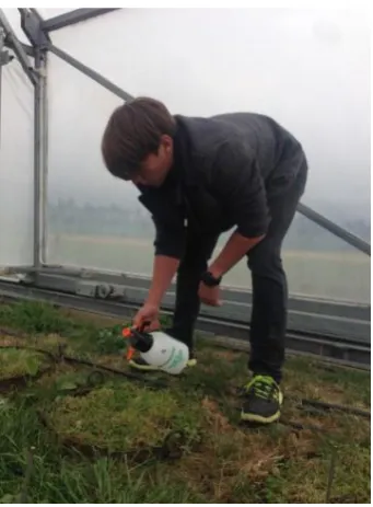
Irrigation season, Experiment 1). KBr was applied as a dissolved solution (equivalent to 2.5 mm) using

a hand-held spray bottle at a rate equivalent to 50 mm/hr. To do this, lysimeters were exposed to

pulsed bromide application over 9 minutes. Tracer application was followed immediately by an

application of irrigation at a volume determined by the lysimeters set treatment (refer to section 3.3.3

Irrigation season, Experiment 1), but deducting the 2.5 mm of irrigation that was applied in the tracer

application. The process was repeated for all twenty-four lysimeters used in the trial. To improve

(26)

Plate 2 Bromide tracer application.

3.3.3 Irrigation season, Experiment 1

The experiment was set as a complete randomised block design. This design was made up of six

treatments, involving three different soil deficits to trigger irrigation and six different irrigation

volumes that equated to two moisture statuses following irrigation (Table 1). Lysimeters were irrigated

at a rate of 50 mm/hr, which is a common rate applied by centre pivot irrigators, as well as roto-rainer

and gun type irrigators (Powers, 2012).

Each treatment was replicated four times to give a total of twenty-four lysimeters. Considering

potential legacy effects (as lysimeters had been used in a previous experiment), two blocks were

dedicated to the lysimeters that received urine in the previous experiment, the remaining two blocks

being dedicated to the lysimeters that did not receive urine. Blocking structure can be seen in Appendix

B.

Table 1 Irrigation treatments and associated moisture status.

Treatment Soil deficit irrigation

trigger

Depth irrigated Moisture status

following irrigation

15/10 15 mm 10 mm 5 mm deficit

15/15 15 mm 15 mm Field capacity

(27)

treatment were assumed to have negligible differences in moisture content and thus irrigated at the

same time. This assumption was deemed acceptable, as it represents common irrigation practice,

where irrigation is triggered based of the average moisture content of a field or farm. The moisture

content averages were based on the readings from sixteen soil moisture sensors, which represent the

four sensors found in each of the four lysimeters within any single treatment. For each depth, the

average soil moisture content was calculated, and these were then summed over the depth of the

lysimeter.

3.3.4 50 mm/hr drainage period, Experiment 2

On the 16th of June, all lysimeters were subject to 250 mm of continuous irrigation (equivalent to

approximately one PV). Irrigation was applied at the same rate as during the irrigation season (50

mm/hr) to leach out bromide residing in the macropores. Considering discrepancies in moisture

content between lysimeters of varying treatments, all lysimeters were irrigated to FC the day before

(15 June) to improve the uniformity of drainage sampling. The infiltration rate of lysimeter twenty-one

was found to be half the rate of the irrigation (50 mm/hr) and the other lysimeters. As a result, this

lysimeter had to be leached for twice as long to allow comparable drainage samples.

3.3.5 2 mm/hr drainage period, Experiment 3

Following completion of Experiment 2, the lysimeters were allowed to drain for c. 24 hours, upon which

drainage had largely ceased. All lysimeters were then subject to a further 500 mm of continuous

irrigation (equivalent to approximately two PV). Irrigation was applied at a rate of 2 mm/hr to leach

out bromide located within the soil matrix. The irrigation period extended from the 17th_{to the 29}th_of

June.

3.4 Lysimeter measurements

3.4.1 Leachate collection and analysis

Drainage water from lysimeters was quantified using tipping spoon data and regular drainage

sampling. Sampling involved measuring the volume of drainage water and taking a 50 mL sample for

chemical analysis.

For Experiment 1, drainage weights were taken at daily intervals following an irrigation event and

continued until drainage had stopped. Sub samples for chemical analysis were taken whenever the

drainage exceeded 50 mL.

The target for Experiments 2 and 3, was to sample leachate at intervals of 25mm. Experiment 2

(28)

irrigation period, as a result of the continual high intensity (50 mm/hr) irrigation. Experiment 3, had

drainage weights and sub samples taken every twelve hours (7:30 am and 7:30 pm).

Considering the number of samples collected across treatments and experiments, only a selection

were analysed for bromide using ion chromatography. From Experiment 1, samples were taken at

times that represented significant drainage for a treatment.

Experiment 2 had 11 samplings over the whole drainage event. Initially, approximately 5 mm of

drainage was analysed (samples 1-5); thereafter, drainage was analysed at c. 50 mm intervals (sample

7, 9 and 11) to determine the shape of the solute breakthrough curve.

Experiment 3 had 24 samplings. Samples were analysed at c. 25 mm drainage intervals (for samples

1-3), then at c. 100 mm drainage intervals (samples 5, 9, 13, 17, 21) and finally sample 24. As with

Experiment 2, this frequency allowed the shape determination of the solute breakthrough curve.

3.4.2 Pasture collection and analysis

Over the course of the investigation, pasture was cut three times as required to prevent significant

disruption to irrigation uniformity on lysimeters. Cuts were made using electric hand shears, and

herbage on all lysimeters was harvested to a standard height of approximately 5 cm (1500 kg DM/ha

residual). Herbage dry weights were measured before removing a subsample for each lysimeter that

incorporated all three pasture cuts. Subsamples were ground and exposed to a water-methanol

extraction before analysis by ion chromatography for bromide.

3.5 Statistical analysis

All data sets were statistically analysed to test for significant treatment effects by conducting an

analysis of variance (ANOVA) using Genstat 13.

Lysimeter 19 (60/60) was not included in the results, as for unknown reasons, herbage died off, and

(29)

Chapter 4 Results

4.1 Soil properties

Soil properties are displayed in Table 2. Total porosity and available water capacity were greatest in

the top 7.5 cm of the soil profile and generally reduced with depth. A significant decrease in hydraulic

conductivity is also apparent with greater soil depth, with an observed 10-fold reduction between the

0-7.5 cm and the 30-40 cm depths under 0.1 and 0.4 kPa suction. Conductivity decreases as suction

increases, which corresponds to the change in active water transmitting pores. Estimates on the

maximum pore size full of water indicate that at 0.1 kPa, water is moving through pores of 3 mm

diameter, decreasing to 0.7 mm under a suction of 0.4 kPa, and down to 0.3 mm under 1 kPa suction.

Using the measurements of total porosity for each depth increment, an estimate of 249 mm was

calculated as the average pore volume (PV) for the 50 cm diameter by 65 cm deep lysimeter soil

columns.

Variability in soil parameters was generally quite low for the examined samples, however, hydraulic

conductivity, especially under low suction, had quite high variability. The standard deviation for the

K0.1_{estimates were almost half the average for the top three sample depths. Variability was observed}

(30)

Table 2 Average hydraulic soil properties. Values in brackets were the calculated standard deviation. Soil properties to the depth of 40 cm were measured from 10x7.5 cm soil cores using pressure plate and tension table apparatus (Carrick, 2009). Soil properties below 40 cm were measured in the field using the volume replacement method (Hedley et al., 2012).

*At the 40 – 65 cm depths the 10 kPa measurement was not directly measured, but is estimated by the volumetric

water content directly measured when the soil was wet to field capacity (Refer to section 3.1 Soil description).

# not measured at this site, but estimated from similar stony soil layers elsewhere.

4.2 Treatment application and wetting and drying cycles, Experiment 1

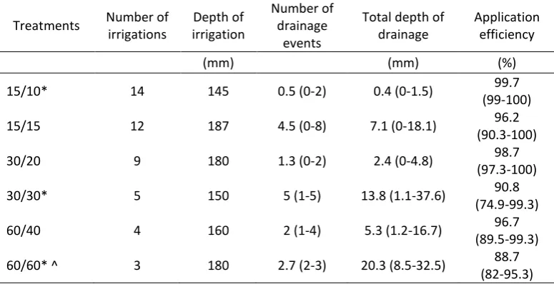
Experiment 1 wetting and drying cycles are presented in Figure 4 for deficit-irrigated treatments and

Figure 5 for field capacity (FC) treatments. Depth of irrigation across all treatments varied from 145

mm (15/10) to 187 mm (15/15), or 0.58 PV and 0.75 PV respectively. Variation arose in the irrigation

applied due to the differences in irrigation return interval. For example, completion of Experiment 1

coincided with the completion of irrigation cycles for the 60/60, 60/40, 30/20 and 15/15 treatments,

but the 15/10 and 30/30 treatments were still mid cycle at the end of Experiment 1, and were hence

an irrigation application behind the other treatments. Irrigation frequency is reflected by the variation

in the degree of soil moisture content fluctuation between treatments, with FC found to be between

150-160 mm total water content for the lysimeters determined by measurements for the initial

pre-experiment lysimeter wetting up (refer to section 3.3.1 Pre-wetting and establishment of antecedent

moisture conditions).

The average treatment application efficiency (AE) defined as the water lost to drainage/amount of

irrigation applied (mm/mm) is presented in Table 3 as a proportion (%). Average AE for all treatments

Volumetric water content Hydraulic conductivity (K)

Depth Stone Bulk

density

Total

porosity @1 kPa

@10 kPa

@1500

kPa AWC K

0.1 kPa _K0.4 kPa _K1 kPa

cm % g cm-3 _% _% _% _% _% _mm/h _mm/h _mm/h

0-7.5 0 (±0) 1.08

(±0.04) 58 (±1.65) 47 (±1.32) 38 (±1.78) 14

(±1.84) 24

120.22 (±57.00) 30.09 (±13.40) 1.42 (±0.61)

7.5-15 0 (±1) 1.33

(±0.04) 49 (±1.55) 40 (±1.59) 34 (±1.53) 16

(±2.46) 18

33.78 (±12.90) 9.58 (±3.28) 1.27 (±0.55)

15-30 0 (±0) 1.36

(±0.07) 48 (±2.38) 38 (±3.48) 31 (±3.00) 15

(±2.34) 16

24.91 (±11.31) 5.8 (±1.79) 0.93 (±0.35)

30-40 2 (±3) 1.47

(±0.04) 44 (±1.17) 35 (±1.56) 29 (±2.17) 16

(±3.04) 13

10.04 (±1.99) 3.06 (±1.17) 0.9 (±0.31)

40-50 60

(±4) 1.99 (±0.09) 25 (±3.23) 10*

(± 1.07) 4# 6

50-65 71

(±1) 2.17 (±0.05) 18 (±1.99) 6*

(± 0.72) 2

(31)

in the 15/15 had five times the number of drainage events and 15 times the quantity of drainage

compared to the 15/10, equating to an average AE difference of 3.5%. The 30/30 had over three times

the number of drainage events and over five times the quantity of drainage compared to the 30/20 on

average. In AE, the 30/20 and 30/30 varied by 7.9%. The 60/60 and 60/40 had a similar number of

drainage events on average (2.7 and 2 respectively), however the 60/60 had nearly four times the

quantity of drainage compared to the 60/40 and a corresponding difference in AE of 8%. Regardless if

treatment was deficit or FC, increasing application volume had a positive correlation with average AE.

AE for FC treatments was in the order of 15/15 (96.2%) > 30/30 (90.8%) > 60/60 (88.7%), deficit

treatments in the order of 15/10 (99.7%) > 30/20 (98.7%) > 60/40 (96.7%).

Lysimeter 9 was the only lysimeter to drain in the 15/10 treatment (Figure 4; Figure 5). The drainage

in the 30/20 treatment was dominated by lysimeters 12 and 24, while lysimeter 20 accounted for most

of the drainage in the 60/40 treatment. All lysimeters in FC treatments generally drained, however

lysimeters 17 (15/15) and 23 (30/30) demonstrated higher, or more numerous drainage events to

other lysimeters within their treatments (Figure 4; Figure 5).

Due to the difference in total depth of irrigation applied for each treatment (Table 3), significance

testing was not viable as any statistical trends may be due to a difference in applied irrigation as

opposed to a treatment effect.

Table 3 Experiment 1 irrigation applied and drainage for the different treatments. Drainage values represent the average of the lysimeter reps within a treatment, whilst values in brackets represent the treatment range, and application efficiency is the proportion of irrigation that wasn’t lost as drainage (average of the lysimeter reps).

Treatments Number of

irrigations Depth of irrigation Number of drainage events

Total depth of drainage

Application efficiency

(mm) (mm) (%)

15/10* 14 145 0.5 (0-2) 0.4 (0-1.5) 99.7

(99-100)

15/15 12 187 4.5 (0-8) 7.1 (0-18.1) 96.2

(90.3-100)

30/20 9 180 1.3 (0-2) 2.4 (0-4.8) 98.7

(97.3-100)

30/30* 5 150 5 (1-5) 13.8 (1.1-37.6) 90.8

(74.9-99.3)

60/40 4 160 2 (1-4) 5.3 (1.2-16.7) 96.7

(89.5-99.3)

60/60* ^ 3 180 2.7 (2-3) 20.3 (8.5-32.5) 88.7

(82-95.3) *Final irrigation not included, as was not a full irrigation.

(32)

(33)

(34)

4.3 Uniformity of drainage events

4.3.1 Experiment 2

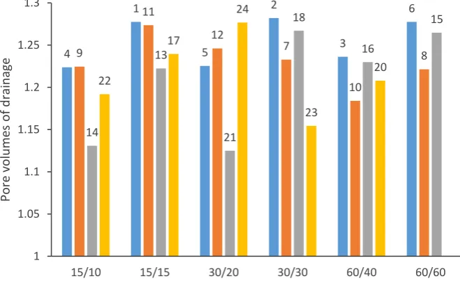
Neither the moisture deficit irrigation trigger (P>0.9) nor the moisture status after irrigation (P>0.05)

had significant effects on the cumulative drainage in Experiment 2, showing there was no residual

effect of the irrigation treatments in Experiment 1 on the quantity of drainage water in Experiment 2.

The relatively low P-value for the effect of moisture status after irrigation (i.e. irrigation to FC or deficit)

is caused by three variable results from lysimeters 14 (15/10), 21 (30/20) and 23 (30/30). Variable

lysimeters had approximately 0.06 PV less drainage (c. 15 mm) compared to other lysimeters in their

treatments (Figure 6). Causation is mostly due to lysimeter variation in soil water properties and the

initial soil water content, with smaller and more variable drainage volume in the first drainage sample

due to lysimeters wetting up to steady state conditions, and variation in the final drainage following

cessation of the irrigation. Any errors in irrigation calibration appear to have only had a minor effect.

Figure 6 Experiment 2 cumulative drainage. Number labels refer to the lysimeter where drainage results were collected from.

4.3.2 Experiment 3

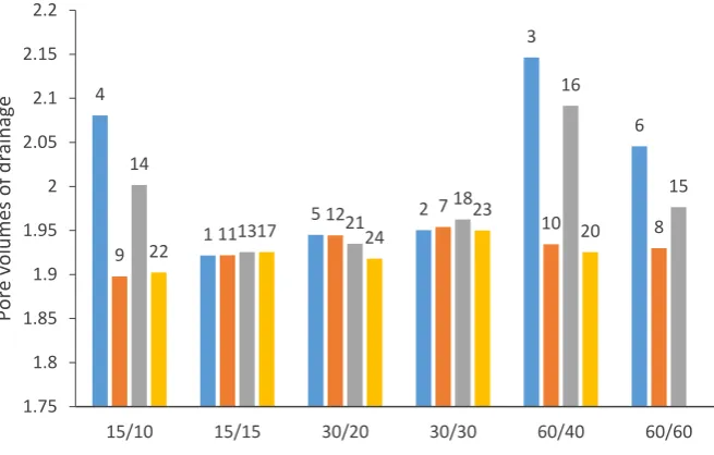
Lysimeters 4 and 14 had about 0.16 PV (c. 40 mm) more drainage compared to other lysimeters in their

treatment (15/10) (Figure 7). Lysimeters 3 and 16 also had about 0.16 PV (c. 40 mm) more drainage to

other lysimeters in their treatment (60/40) (Figure 7). These higher drainages may be due to lysimeter

variation, but is likely as a result of calibration errors for irrigation or a change in solenoid response

over time. This arises as the low 2 mm/hr rate was the limit of precision that could be achieved with

the irrigation system, especially over such a prolonged drainage event where minor drips can cause

4 1 5 2 3 6 9 11 12 7 10 8 14 13 21 18 16 15 22 17 24 23 20 1 1.05 1.1 1.15 1.2 1.25 1.3

15/10 15/15 30/20 30/30 60/40 60/60