© Shiraz University
A GENERALIZED APPROACH FOR MODEL-BASED SPEAKER-DEPENDENT
SINGLE CHANNEL SPEECH SEPARATION*
M. H. RADFAR1, ** A. SAYADIYAN1, AND R. M. DANSEREAU2
1Dept. of Electrical Engineering, Amirkabir University of Technology, Tehran, I. R. of Iran,15875-4413 Email: [email protected]
2Dept. of Systems and Computer Engineering, Carleton University, Ottawa, Ontario, Canada, K1S 5B6 Abstract– In this paper, we present a new technique for separating two speech signals received from one microphone or one communication channel. In this special case, the separation problem is too ill-conditioned to be handled with common blind source separation techniques. The proposed technique is a generalized approach to model-based speaker-dependent single channel speech separation techniques in which a priori knowledge of the underlying speakers is used to separate speech signals. The proposed technique not only preserves the advantages of model-based speaker dependent single channel speech separation algorithms (i.e. high separability), but also is able to separate the speech signals of an unlimited number of speakers given the speakers' models (i.e. generality). The whole algorithm consists of three stages: classification, identification, and separation. The identities of speakers speech signals form the mixed signal are first determined at the classification and identification stages. Identified speakers' model is then used to separate the underlying signals using a novel approach consisting of Gaussian mixture modeling, maximum likelihood estimation and Wiener filtering. Evaluation results conducted on a database consisting of 100 mixed speech signals with target-to-interference ratios (TIR) ranging from -9 dB to +9 dB show significant performance improvements over those techniques which use a single model for separation.
Keywords– Source separation, single channel speech separation, speaker identification, model-based single channel speech separation, Wiener filtering
1. INTRODUCTION
The human auditory system is able to pick one conversation out of dozens in a crowded room. This is a capability that no artificial system comes close to matching. Recently, many efforts have been carried out to mimic this fantastic human ability. Inspired by this, the separation of two speech signals received from one communication channel is a challenging topic in the speech processing context. Currently, blind source separation techniques [1]-[7] are commonly used in the speech separation problem. In fact, if the requirements of BSS methods are satisfied, these techniques separate out speech signals with higher accuracy in comparison with other state-of-the art techniques such as computational auditory scene analysis (CASA) [7]. One of these requirements is that the number of observations must be at least equal to the number of sources, a condition which is not held when we have just one microphone and two speakers. This drawback, which significantly confines the usefulness of the BSS techniques in the problem at hand, can be explained as follows. In the BSS context, the separation of I source speech signals when we have access to J observation signals can be formulated as
t
t AX
Y =
where t T J t j t
t =[y , ,y , ,y ]
Y 1 K K ,
T t I t i t
t =[x , ,x , ,x ]
X 1 K K and A=[ai,j]I,J is an (I×J) instantaneous
mixing matrix which shows the relative position of the sources from the observations. Also, vectors
N n t j t
j ={y (n)}=1
y and N
n t i t
i ={x(n)}=1
x for j=1,2,K,J and i=1,2,K,I represent N-dimensional vectors of the jth observation and ithsource signals, respectively. Additionally, [⋅]T denotes the transpose operation
and the superscript t indicates that the signals are in the time domain. When the number of observations is equal or greater than the number of sources (J> ), the solution to the separation problem is simply I obtained by estimating the inverse of the mixing matrix, i.e.
W
=
A
-1, and left multiplying both sides ofthe above equation byW . Many solutions have, so far, been proposed for determining the mixing matrix and quite satisfactory results have been reported [1]-[6].
However, when the number of observations is less than the number of sources (J < ), (e.g.I J=1 and 2I = for the case discussed in this paper) the mixing matrix is non-invertible such that the problem becomes too ill-conditioned to be solved using common BSS techniques. In this case, we need auxiliary information (e.g. a priori knowledge of sources) to solve the problem. This problem is commonly referred to as model-based single channel speech separation and has recently become a hot topic in the signal processing realm [8]. Although several solutions to this crux problem have been proposed by including the a priori knowledge of underlying speakers into the separation system [9]-[24], the problem has still remained a challenge such that current proposed algorithms deliver acceptable quality only in special cases. Generally, single channel model-based speech separation techniques are categorized into two classes: time domain and frequency domain.
In time domain techniques [9]-[13] each source is decomposed into independent basis functions in the training phase. The basis functions of each source are learnt from a training data set based on independent component analysis approaches. Then the trained basis functions along with the constraint imposed by the linearity of sources in the time domain are used to estimate the individual speech signals via a maximum likelihood optimization. While the techniques perform well when the speech signal is mixed with other sounds such as music, separability reduces significantly when the mixture consists of two speech signals since the learnt basis functions of two speakers overlap greatly. In frequency domain techniques [14]-[19], first a statistical model is fitted to the log spectral vectors of each speaker. Then, the two speaker models are combined to model the mixed signal. Finally, in the test phase, the states that best match the mixed signal are decoded based on some criteria (e.g., minimum mean square error, likelihood ratio).
In this paper, we propose a new model-based single channel technique that not only takes on the advantages of speaker-dependent model-based approaches but also is able to separate the speech signals even if they come from unknown speakers. The system can be adapted to as many speakers as possible given a training data set of the speakers. The proposed technique consists of three stages: classification, identification, and separation. The algorithm first recognizes the underlying speakers, and then the trained models of the selected speakers are used in the separation process. We apply a new separation technique which employs Gaussian mixture modeling, maximum likelihood estimation and Wiener filtering to separate the speech signals. The classification stage is based on a new algorithm known as the harmonic matching classifier followed by the identification stage. We evaluate the performance of the whole system as well as the performance of each stage separately. Results show the proposed technique outperforms those techniques which apply a single trained model for all speakers.
The remainder of this paper is organized as follows. In Section 2, we present a brief overview of the whole system. In Section 3, we discuss the classification stage. The identification process is given in Section 4 followed by the separation system which is explored in Section 4. Experimental results are reported in Section 5 and, finally, conclusions are discussed in Section 6.
2. MODEL OVERVIEW
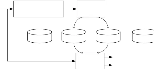
In this section, we present a brief overview of the proposed technique and in the subsequent sections we elaborate on the details of the algorithm. Fig. 1 shows the system’s block diagram which consists of three stages: classification, identification, and separation.
Fig. 1. Schematic diagram of the proposed system. The system consists of classification, identification, and separation stages
The extracted features (i.e U-V frames) are then transformed to the mel frequency cepstral coefficients (MFCC) and passed to the identification stage. The task of the identification stage is to identify the two speakers among the N speakers. We apply a speaker identification algorithm based on the techniques known as VQ-based speaker identification [33]-[35]. These techniques, however, are designed to identify one speaker among the N speakers. Therefore, we modify the VQ-based speaker identification algorithms to be able to recognize two speakers among the N speakers.
Finally, the last stage of the proposed algorithm is intended to separate the underlying speech signals of the identified speakers. In this stage, we introduce a new technique which applies Gaussian mixture modeling, maximum likelihood estimation, and Wiener filtering to separate speech signals. A block diagram of the proposed separation algorithm is shown in Fig. 2. In this stage, the power spectrum density (PSD) of the underlying speech signals is estimated in a maximum likelihood estimation process at the frame level. Then the estimated PSDs are fed into the Wiener filter so as to estimate the speech signals. In the following sections we present the details of these algorithms.
GMM(i)
...
GMM(j)
...
ML Estimator
x’i(t)
x’j(t) Mixed signal
xmix(t)
Fig. 2. Block diagram of the separation stage which separates the underlying speech
3. CLASSIFICATION STAGE
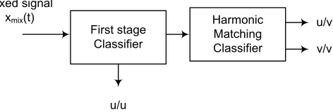
As mentioned earlier the task of the classification stage is to recognize the U-V frames which are appropriate for speaker identification. Fig. 3 shows a schematic of the proposed classifier which consists of two stages. At the first stage, we distinguish the U U frames from V-V and U-V frames, and at the second stage the U-V frames are recognized from the V-V frames.
Harmonic Matching Classifier Mixed signal
xmix(t)
u/u
v/v u/v First stage
Classifier
Fig. 3. Block diagram of the classification stage consisting of two parts: the U-U classifier and the harmonic match classifier to recognize U-V from V-V
distinguish the V-V frames from the U-V frames. Recently, this topic has been dubbed in speech separation literature as usable speech detection [36]. The main application of usable speech detection is in the co-channel speaker identification problem where the aim is to recognize the U-V frames whereby speaker identities are recognized. Several approaches have been proposed for distinguishing U-V frames from V-V frames, namely using the spectral autocorrelation peak valley ratio (SAPVR) criterion [37], nonlinear speech processing [38], wavelet analysis [39], Bayesian classifiers [40], or pitch information [41]. In this paper, we introduce a new technique which we call the harmonic matching classifier (HMC). The algorithm is explained in the following paragraph.
As mentioned earlier, the main characteristic of voiced frames, i.e. periodic nature, are preserved when a voiced frame interacts with an unvoiced frame in the mixed speech signal. In this case, we can fit a harmonic model to a U-V analysis frame with a modeling error which is considerably less than that of fitting a harmonic model to a V-V frame. In the latter case, harmonic modeling just covers the spectral peaks belonging to one speaker and thus leads to a high modeling error. The detailed algorithm for extracting the U-V frames is described in Table I. In this algorithm, |Xt (ω)|2
mix denotes the spectrum of the th
t mixed signal frame. Moreover, the harmonic model is represented by
‡”
) (
1 2
2 ( )
i
i
L
l
i
l W l
A ω
ω ω ω
=
− , in which
the applied spectrum window, W(ω), is repeated at integer multiples of the fundamental frequency ωi
with an amplitude proportional to i ω
l
A . Also L(ωi)represents the number of harmonics in the speech bandwidth. For each frame we find the best harmonic match and compute the model error. If the corresponding error is less than the thresholdσ, the frame is classified as a U-V frame, otherwise it is a V-V frame. Using a training data set we obtained the best value for = ({ }=)
T t t
e mean
σ 1 , where
t
e is the model error for the frame t (see Table 1 for more details). We report the performance of the harmonic matching classifier along with a comparison with a state-of-the-art technique in Section 5. Finally, it should be noted that although the silence segment in a classification process is desirable, but in this paper we consider the silence segments as a special case of unvoiced segments.
Table 1. Harmonic matching classifier
4. IDENTIFICATION STAGE
Let }Θ={1,2,K,S be a group of speakers among whom we wish to identify the two speaker identities given a mixed utterance. Having the training data set for each speaker, we first partition the feature space (MFCCs) of each speaker into K partitions using the Linde-Buzo-Gray (LBG) vector quantization algorithm [42]. Then, partition centers i
k
c (known as codewords) are extracted and form the speaker i codebookΨ ={ , , , i}
K i
i c c
c
i
K
2
1 . Each codeword, in turn, contains the first M MFCCs (excluding
the first one) that is, =[ci(),ci( ), ,ci(M)]T K
2 1
i
c , where [⋅]Tdenotes the transpose operation.
• Find error introduced by fitting a harmonic model to the tth mixed analysis frame
) (
) (
min
‡”
* i
) L(ω
l lω
t mix
t X A W ω lω
e i i
i
− −
=
= 2 1
2 2
ω ω
• V-V and U-V classification ifet ¡Üσ
frame ¸ U-V else
frame ¸V-V end
• Repeat the algorithm for all frames
Accordingly, performing quantization on the training data set of all speakers we obtain the set } , , { =
Ψ C C CS
K
2
1 consisting of all speakers' codebooks. Now the objective is to find two speakers by
minimizing the following criteria
‡”
¸ ¸ ) , ( min min arg* t U V
i k t mix k i D − Θ c
c (1)
‡”
¸ } { -¸ ) , ( min min arg * * V U t j k t mix k i j D − Θ cc (2)
where i* and j*are selected speakers and t mix
c mix is the MFCC vector extracted from the tth U-V mixed
analysis frame. Additionally, ( , i)
k t mix
D c c represents the Euclidean distance between the vectors t mix
c and
i k
c as defined by
∑
= − = M m i k t mix i k tmix c m c m
D 1 2 )) ( ) ( ( ) ,
(c c (3)
Equations (1) and (2) can be interpreted as follows. First, for those frames recognized as the U-V frames in the mixed speech signal, a search is done through all codewords (k=1:K) of all speakers' codebooks (i=1:S). The speaker who obtains the minimum distortion measure for all U-V frames is selected as the first underlying speaker. A similar process is again performed to select the second underlying speaker but the selected speaker from the first search process is excluded from the searching process.
4. SEPARATION STAGE
a) Relation between the log spectra vectors
In this subsection, we assume that the two speakers whose utterances form the mixed speech signal were specified from the identification stage. Let x1(t) and x2(t) be the speech signal of speaker one and two, respectively. An N-dimensional vector of samples of x1(t) and x2(t) at time m are denoted by
T t
t t
t(m) [x(m),x(m 1), ,x(m N 1)]
1 1
1
1 = + K − +
x (4)
T t
t t
t(m) [x (m),x (m 1), ,x (m N 1)]
2 2
2
2 = + K − +
x (5)
where [⋅]T denotes the transpose operation and the superscript t denotes the time domain notation. We
assume that the observed signal yt(m) is the sum of the speech signals of the two speakers as follows
). ( + ) ( = )
(m t m t m
t
2
1 x
x
y (6)
We next form the following vectors
T t
D( (m))| x( ), ,x( ), ,x(D)
F
(| )=[ ]
log
= 10 1 1 1 1
1 x 1 K 2 K
x (7)
T t
D( (m))| x( ), ,x( ), ,x(D)
F )=[ ]
(| log
= 10 2 2 2 2
2 x 1 K 2 K
x (8)
T t
D( (m))|) y( ), ,y( ), ,y(D)
(|F =[ ]
log
= 10 y 1 K 2 K
y (9)
where x1, x2, and y denote the D-dimensional log spectral vectors of speaker one and speaker two, the
spectrum of the mixed signal is nearly the element wise maximum of the log spectrum of the two underlying signals. Mathematically, the approximation can be formulated as follows
T D x D x d x d x x x
Max( , ) [max( (), ( )), ,max( ( ), ( )), ,max( ( ), ( ))]
ˆ= x1 x2 = 11 2 1 K 1 2 K 1 2
y (10)
Hence, yˆ is an approximation to y with reasonable accuracy. It should be noted that MFFC coefficients used in the identification stage cannot be used in the separation stage for two reasons. First, the MFCC is a non linear feature such that we cannot re-synthesize the speech signal from the MFCC coefficients. For this reason, although MFFC is widely used in classification based techniques such as speech or speaker recognition, we cannot use it for re-synthesizing a speech signal. Second, there is no straightforward relationship between the MMFSs of the mixture and those of the underlying signals.
b) Maximum likelihood estimator
We next model the probability density function of the ith speaker's log spectral vectors by a mixture of
Ki Gaussian densities in the following form
} , { ¸ ) , , ( )
( , , , 12
1
i N
c
f i x k x k
K
k x k
i i i
i i
i x x U
x
∑
µ=
= (11)
where cxi,k represents the a priori probability for the
th
k Gaussian in the mixture and satisfies
‡”
kcxi,k =1, and | | ) ( )) ( ) ( exp( ) , , ( , , , , , k x D k x i k x T k x i x k x i i i i i i i N U x U x U x π µ µ µ 2 21 − 1 −
− =
−
(12)
represents a D-dimensional normal density function with the mean vector µxi,k and covariance
matrixUxi,k. The D-variant Gaussians are assumed to be diagonal covariant to reduce the order of
computation. This assumption enables us to represent the multivariate Gaussian as the product of D uni-variant Gaussians given by
¡Ç
) ( ) ( ) ( ) ( exp ) ( , , , , Dd x k
k x k x i K k k x i x d d d d x c f i i i i i i 1 2 1 2 2 1 = = − − =
∑
σ π σ µx (13)
where, )xi(d , µxi,k(d) and σxi,k(d)
2 are the dth component of i
x, dth component of the mean vector, and
the dth element on the diagonal of the covariance matrix, respectively.
As mentioned earlier, the log spectral vectors of the mixed signal are almost exactly the maximum element-wise components of the log spectral vectors of the underlying signal, that is
). , max(
¡Ö x1 x2
y (14)
The cumulative distribution function (CDF) of the mixed log spectral vectors Fy(y) is given by
) , ( = )
(y x1,x2 y y
y F
F (15)
where )Fx1,x2(y,y is the joint CDF of the random vectors x1 and x2. Since the speech signals of the two
speakers are independent, then
). ( × ) ( = )
(y y y
2
1 x
x
y F F
Thus )fy(y is obtained by differentiating both sides of Eq. (16) to give ). ( ) ( + ) ( ) ( = )
(y y y y y
1 2 2
1 x x x
x
y f F f F
f (17)
The CDF to express (y) i
x
F is obtained by
∫ ∑
∫
−∞ = = ∞ − − − × = = ( ) 1 2 , , , 1,
¡Ç
) )) ( ) ( ( 2 1 exp( 2 ) ( 1 ) ( )
( y d
D d d k x k x d k x K k k x y x x d d d d c d f F i i i i i i
i
σ
ξ
µ
ξ
π
σ
ξ
ξ
y (18)
Since the integration of the sum of the exponential functions is identical to the sum of the integral of exponentials as well as assuming a diagonal covariance matrix for the distributions, we conclude that
¡Ç
( ), , , , ) ) ) ( ) ( ( exp( ) ( ) ( D d d y d k x k x d k x K
k xk
x d d d d c F i i i i i i 1 2 1 2 1 2 1 = −∞ = − − ×
=
∑
∫
ξσ µ ξ π
σ
y (19)
The term in the bracket in Eq. 19 is often expressed in terms of the error function
∫
−= α ν ν
π
α 0 2
2 1 2
1
d
erf( ) exp( ) (20)
Thus, we conclude that
¡Ç
[ ( ( )) ] ) ( , , D d k x K k kx erf z d
c F i i i i 1 1 2 1 = = + =
∑
yx (21)
where } , { ¸ ) ( ) ( ) ( ) ( , ,
, i 12
d d d y d z k x k x k x i i i σ µ −
= (22)
Finally, we obtain the PDF of the log spectral vectors of the mixed signal by substituting Eq. (13) and Eq. (21) into Eq. (17) to give
× + × + × + × × = = = = =
∑∑
¡Ç
¡Ç
1 2 , , 2 1 2 , 1 2 , , 2 1 2 , 1 1 , , )) ( 2 1 exp( ) 2 1 )) ( ( ( )) ( 2 ( )) ( 2 1 exp( ) 2 1 )) ( ( ( )) ( 2 ( ) ( 2 1 2 1 2 1 1 2 2 1 D d l x k x l x D d k x l x k x K k K l l x k x d z d z erf d d z d z erf d c c fπσ
πσ
y y (23)Equation (23) gives the PDF of log spectral vectors for the mixed signal in terms of the mean and variance of the log spectral vectors of the underlying signals.
Now we apply fy(y) in a maximum likelihood framework to estimate the parameters of the underlying signals. The main objective of the Maximum Likelihood estimator is to find the kth Gaussian in
) ;
( 1
1 1 λx
fx x and the l
th Gaussian in ( ; )
2
2 2 λx
fx x such that fy(y) is maximized. The estimator is given by
{ }
ˆ,ˆ =argmax ( | ,), kl
θ
ML f θ
l k
l k
y
y (24)
where
{
x k x l x k x l}
l
k,
µ
1, ,µ
2, ,σ
1, ,σ
2,θ
= (25)c) Wiener filtering
From the Wiener filtering theory [45], we know that the optimal filter for stationary processes that can estimate a signal corrupted by noise (for our case the term noise means the other speaker's signal) is given by
) ( ) ( ) (
) ( ¡Ö
)) ( (
2 1
1
2
1
ω
ω
ω
ω
y x x
x t
D S
S S
S m
F
+
x (26)
where ( )
1
ω
x
S , ( )
2
ω
x
S , and Sy(ω) are the power spectral densities associated with speaker one, speaker two, and the mixed signal, respectively. Approximation to F ( 2t(m))2
D x is also obtained in a similar way.
In Eq. (26), however, we have no access to the speakers' PSDs, so we replace them by the estimated log spectral vectors, i.e. x,k
1
µ
and x ,l2
µ
, obtained from the previous subsection (Eq. (25)). Thus, we have) ( 10
10 10 ¡Ö
)) (
( 2 ( ) 2 ( )
) ( 2 2
1 ,
2 ,
1 , 1
ω
ω µ ωµ
ω µ
y t
D m S
F
k x l
x
l x
+
x (27)
Finally, the estimated signals are obtained in the time domain by
(
( ( )).Ú ( ( )))
¸{1,2} )(
ˆ m F 1 F x m F y m i
x t
D t
i D D t
i = (28)
where FD−1 denotes the inverse Fourier transform and ÚF ( t(m))
D y is the phase of the Fourier transform
of the mixed signal. In this way, we obtain an estimate of t(m)
i
x . It should be noted that it is common to use the phase of the STFT of the mixed signal for reconstructing the individual signals [14]-[16], [27] as it has no palpable effect on the quality of the separated signals. Recently it has been shown that the phase of the short-time Fourier transform has valuable perceptual information when the speech signal is analyzed with a window of long duration, i.e., >1 sec. [46]. To the best of our knowledge no technique has been proposed to extract the individual phase values from the mixed phase.
5. EXPERIMENTAL RESULTS
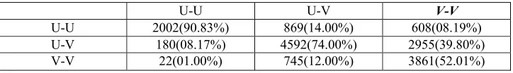
We first conduct experiments in order to evaluate the performance of the classification stage. In order to put the results into perspective, we compare the voicing state classification results of our model with that of Wu et al. [47]. The technique proposed in [47] is, in fact, a multi-pitch tracking system which detects not only the underlying speakers' pitch values, but also voicing states. We set the Wu's multi-pitch tracking parameters from the package they provided and compare the results with our approach. Table 2 shows how the voiced and unvoiced frames interact in the 100 mixed speech signals. As the table shows 13.92, 39.19, and 46.89 percent of the mixed frames belong to U-U, U-V, and V-V states, respectively. In Tables 3 and 4 we present the confusion matrix for the classification results obtained from our approach and the method proposed in [47], respectively. Each diagonal entry of the matrix shows the number of paired frames that are classified correctly and off-diagonal entries show the number of misclassified paired frames. From Tables 3 and 4 we can observe that in our system with respect to the Wu's approach, the classification performance for the U-U, U-V, and V-V states, on average, have improved 8, 2, and 20 percentage respectively. The most difficult task in both our system and Wu’s approach is to recognize the U-V frames from V-V frames, though our system has significantly decreased the error rate for this case. We noticed that two sources of error occur in the classifier. The first one is mainly due to the transitional regions where determining the voicing state, even in the single speech case, is a difficult task. The second source of misclassification happens when the pitch values of the underlying signals lie within the same range. It should be noted that, to the best of our knowledge, no method has so far been proposed to handle these circumstances.
Table 2. Interaction of states in the data base
U-U U-V V-V 2204(13.92%) 6206(39.19%) 7424(46.98%)
Table 3. Confusion matrix of voicing state classification for the method proposed in [47]
U-U U-V V-V
U-U 2174(98.64%) 572(09.22%) 223(03.00%)
U-V 20(00.91%) 4762(76.73%) 1856(25.00%)
V-V 10(00.45%) 872(14.05%) 5345(72.00%)
Table 4. Confusion matrix of voicing state classification for the proposed method in this paper
U-U U-V V-V
U-U 2002(90.83%) 869(14.00%) 608(08.19%)
U-V 180(08.17%) 4592(74.00%) 2955(39.80%)
V-V 22(01.00%) 745(12.00%) 3861(52.01%)
In order to evaluate the accuracy of the identification stage, we measure the correct speaker identification rate of the system for two groups of input features. First, with the MFCC coefficients of the U-V frames obtained from the classification stage; and second with the MFCC coefficients of all frames (without classification). 100 test mixed signals are fed to the speaker ID stage and the percentages of times in which the target and interference are correctly identified are computed. Figures 4 and 5 show the correct speaker ID rate for the target and interferences with and without the U-V frame extraction. We observe that the correct identification rate obtained from the U-V features, on average, outperforms that of the non-classified features.
the speaker ID rate has a direct relation with the length of the test utterance such that the more test speech applied, the better the identification performance obtained [49]. Let c
s
n1 be the number of detected mixed frames in which speaker one is in the V state and speaker two in the U state. Also let o
s
n1 be the number of original voiced frames of speaker one. If we assume that speaker one is the target signal, then when SSR
increases, o
s c
s n
n 1
1 ¨ . Thus the performance of the system with/without classification becomes identical. The same justification can be made for the interference signal. Accordingly, as the TIR increases or
decreases from zero the target or interference becomes the dominant speaker (i.e. o
s c
s n
n1 ¨ 1), and consequently the performance of with/without classification approaches the same values.
Fig. 4, Correct speaker ID rate versus TIR ratio for target speech signals
-9 -6 -3 0 3 6 9
0 10 20 30 40 50 60 70 80 90 100
TIR (dB)
S
peak
er
I
D
R
at
e (
%
)
Classification--Interference No classification--Interference
Fig. 5. Correct speaker ID rate versus TIR ratio for interference speech signals
The last and the most important stage of the system is the separation stage. In this stage, we first model the spectral space of each speaker using a mixture of Gaussian densities. The spectral vectors are extracted from the segments obtained by applying a Hamming window with a length of 52 msec at a frame
-9 -6 -3 0 3 6 9
0 1 2 3 4 5 6 7 8 9 100
TIR (dB)
S
pea
ker
ID Ra
te
(%
)
rate equal to 10 msec. In [50], we showed that for model based single channel speech separation algorithms, this window length leads to the optimal separation performance. Then, a 512-point discrete Fourier transform (D=512) is applied to the windowed segments, resulting in spectral vectors of dimension 256 (symmetric part was discarded). In order to fit a mixture of Gaussian densities to each speaker’s feature space, we first tried to apply the Expectation-Maximization approach which is commonly used for GMM training. Unfortunately we encountered two problems that caused the training procedure to be intractable. First, the feature vector's dimension is remarkably higher than that used in other applications (e.g. Speech recognition, identification) where a vector with 20-40 elements is applied. Second, we need to train a GMM with a large number of elements (we use 256 elements) since we want to recover the underlying speech signals from the mean vectors of Gaussians. Hence, we found that for 15 minute training data it is time consuming to train a GMM with the above specifications using the available software. Therefore, we use a semi-continuous GMM model trained in the following manner. We assume that all components are equal probable. In addition, the Gaussians mean vectors are obtained using an 8 bit-codebook and Gaussians covariance matrixes are obtained from computing the sample covariance matrix of each cluster. To further decrease the computational burden, we just use the diagonal components of the sample covariance matrixes.
In order to show the superiority of speaker-dependent separation modeling over speaker-independent separation modeling, we also fit a GMM to the training data of all speakers. We quantify the degree of the separability by computing the SNR between the separated and the original signals in the time domain. The SNR value for the separated speech signal of the ith speaker is defined as
N n
n x n x
n x
n i i
n i
i ] , , ,
) ) ( ˆ ) ( (
) ( [
log SNR
‡”
‡”
K 2 1
10 2
2
10 + =
= (29)
where )xi(n and xˆi(n) are the original and separated speech signals of length N, respectively.
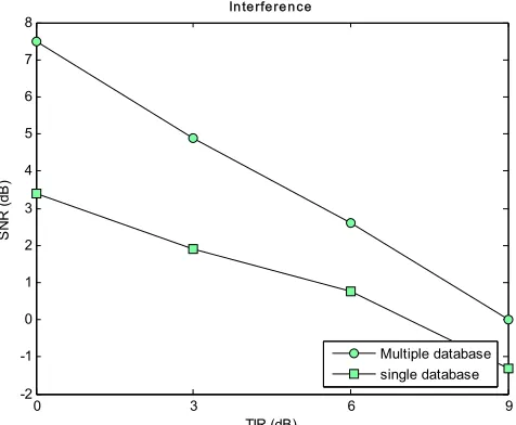
Figures 6 and 7 show the SNR results versus the TIR ratio averaged over 20 separated utterances for the target and interference speeches, respectively. The circled and squared lines show the results for speaker-dependent modeling (multiple database) and speaker-independent modeling (single database), respectively. The results are shown for both target (Fig. 6) and interference (Fig. 7) speeches. From Figs. 6 and 7, we observe that, on average, there is a 3.5 dB performance gain over the speaker-independent scenario. This improvement is remarkable in current single channel speech separation techniques.
0 3 6 9
3 4 5 6 7 8 9 10
TIR (dB)
SN
R
(
dB
)
Target
Multiple database single database
0 3 6 9 -2
-1 0 1 2 3 4 5 6 7 8
TIR (dB)
S
NR (d
B
)
In terfere n ce
Multiple database single database
Fig. 7. SNR versus TIR ratio averaged over separated interferences speech signals
6. CONCLUSIONS
In this paper, we have presented a new model-based single channel speech separation technique. This technique can be effectively applied to separate two speech signals from their mixture where the common single channel separation techniques fail to handle the problem. The proposed technique not only preserves the advantages of speaker dependent single channel speech separation algorithms, but is also able to separate the speech signals of an unlimited number of speakers given the speakers' models. The speaker databases can be augmented into the system in an adaptation phase. The proposed technique consists of three stages: classification, identification, and separation. The speakers' identities are first determined using the classification and identification stages. Then, the identified speakers' models are used to separate the underlying signals. The performance of classification, identification and separation were evaluated and compared with current algorithms. The obtained results also support the idea that the human auditory system uses a priori knowledge about the concurrent sounds to separate them. We believe the next step in this research should be to first improve the identification accuracy and second, adapt the system for a new speaker using the prevalent speaker adaptation techniques applied in speech recognition.
Acknowledgment- The authors would like to thank the Iran Ministry of Science and Research and the
Natural Sciences and Engineering Research Council (NSERC) of Canada which partially funded this research.
REFERENCES
1. Jutten, C. & Herault, J. (1991). Blind separation of sources, part i: An adaptive algorithm based on neuromimetic architecture. Signal Processing, 24, 1–10.
2. Common, P. (1994). Independent component analysis, a new concept? Signal Processing, 36, 287–314.
3. Bell, A. J. & Sejnowski, T. J. (1995). An information-maximization approach to blind separation and blind deconvolution. Neural Computation, 7, 1129–1159.
4. Amari, S. I. & Cardoso, J. F. (1997). Blind source separation–semiparametric statistical approach. IEEE Trans. Signal Processing, 45(11), 2692–2700.
6. Burel, G. (1992). Blind separation of sources: a nonlinear neural algorithm. Neural Networks, 5, 937–947. 7. van der Kouwe, A. J. W., Wang, D. L. & Brown, G. J. (2001). A comparison of auditory and blind separation
techniques for speech segregation. IEEE Trans. Speech and Audio Processing, 9(3), 189–195.
8. Ellis, D. (2006). Model-based scene analysis. in Computational Auditory Scene Analysis: Principles, Algorithms, and Applications, D. W. G. Brown, Ed. Wiley/IEEE Press in press.
9. Jang, G. J. & Lee, T. W. (2003). A probabilistic approach to single channel source separation. in Proc. Advances in Neural Inform. Process. Systems, 1173–1180.
10. [10] Fevotte, C. & Godsill, S. J. (2005). A Bayesian approach for blind separation of sparse sources. IEEE Trans. on Speech and Audio Processing, 4(99), 1–15.
11. Girolami, M. (2001). A variational method for learning sparse and overcomplete representations. Neural Computation, 13(11), 2517–2532.
12. Lee, T. W., Lewicki, M. S., Girolami, M. & Sejnowski, T. J. (1999). Blind source separation of more sources than mixtures using overcomplete representations. IEEE Signal Processing Letters, 6(4), 87– 90.
13. Beierholm, T., Pedersen, B. D. & Winther, O. (2004). Low complexity Bayesian single channel source separation. in Proc. ICASSP–04, 5, 529–532.
14. Roweis, S. (2000). One microphone source separation. in Proc. Neural Inf. Process. Syst., 793–799.
15. Reyes-Gomez, M. J., Ellis, D. & Jojic, N. (2004). Multiband audio modeling for single channel acoustic source separation. Proc. ICASSP–04, 5, 641–644.
16. Reddy, A. M. & Raj, B. (2004). A minimum mean squared error estimator for single channel speaker separation.
in INTERSPEECH, 2445–2448.
17. Kristjansson, T., Attias, H. & Hershey, J. (2004). Single microphone source separation using high resolution signal reconstruction. Proc. ICASSP–05, 817–820.
18. Rowies, S. T. (2003). Factorial models and refiltering for speech separation and denoising. EUROSPEECH–03, 7, 1009–1012.
19. Radfar, M. H., Dansereau, R. M. & Sayadiyan, A. (2006). A novel low complexity VQ-based single channel speech separation technique. into appear in IEEE International Symposium on Signal Processing and Information Technology.
20. Wan, E. A. & Nelson, A. (1997). Neural dual extended kalman filtering: Applications in speech enhancement and monaural blind signal separation. IEEE Proc. Neural Networks for Signal Processing, 466–475.
21. Hopgood, J. R. & Rayner, P. J. W. (2003). Single channel non-stationary stochastic signal separation using linear time-varying filters. IEEE Trans. Acoustics, Speech, and Signal Process, 51(7), 1793–1752.
22. Balan, R., Jourjine, A. & Rosca, J. (1999). Ar processes and sources can be reconstructed from degenerative mixtures. Proc. ICA-99, 467–472.
23. Radfar, M. H., Dansereau, R. M. & Sayadiyan, A. (2006). A joint probabilistic-deterministic approach using source-filter modeling of speech signal for single channel speech separation. Proc. IEEE MLSP-06, 47–52. 24. Radfar, M. H., Dansereau, R. M. & Sayadiyan, A. (2006). Performance evaluation of three features for
model-based single channel speech separation problem. Interspeech 2006, Intern. Conf. on Spoken Language Processing (ICSLP’2006 Pittsburgh), 2610–2613.
25. Bregman, A. S. (1994). Computational auditory scene analysis. Cambridge MA: MIT Press.
26. Brown, G. J. & Cooke, M. (1994). Computational auditory scene analysis. Computer Speech and Language, 8(4), 297–336.
27. Hu, G. & Wang, D. (2004). Monaural speech segregation based on pitch tracking and amplitude modulation.
IEEE Trans. Neural Networks, 15(5), 1135–1150.
29. Virtanen, T. & Klapuri, A. (2000). Separation of harmonic sound sources using sinusoidal modeling. Proc. ICASSP–2000, 765–768.
30. Quatieri, T. F. & Danisewicz, R. G. (1990). An approach to co-channel talker interference suppression using a sinusoidal model for speech. IEEE Trans. Acoustics, Speech, and Signal Process, 38, 56–69.
31. Radfar, M. H., Sayadiyan, A. & Dansereau, R. M. (2006). Monaural multipitch tracking using joint mean square error harmonic modelling and sinusoidal spectrogram. submitted to Speech Communication.
32. Talkin, D. (1995). Robust pitch tracking. in speech coding and synthesis. W. Kleijn and K. Paliwal, Eds. Elsevier.
33. Kinnunen, T., Karpov, E. & Franti, P. (2006). Real-time speaker identification and verification. IEEE Trans. Speech Audio Processing, 14(1), 277–288.
34. Jialong, H., Li, L. & Palm, G. (1999). A discriminative training algorithm for VQ-based speaker identification.
IEEE Trans. Speech Audio Processing, 7(3), 353–356.
35. Soong, F., Rosenberg, A., Rabiner, L. & Juang, B. (1985). A vector quantization approach to speaker recognition. Proc. ICASSP-85, 10, 387–390.
36. Yantorno, R. E. (1999). Co-channel speech study, Air Force Office of Scientific Research Speech Processing Lab Rome Labs. Report for Summer Research Faculty Program.
37. Chandra, N. & Yantorno, R. E. (2002). Usable speech detection using the modified spectral autocorrelation peak to valley ratio using the LPC residual. Proc. 4th IASTED–02, 146–149.
38. Mahgoub, Y. & Dansereau, R. (2005). Voicing-state classification of cochannel speech using nonlinear state-space reconstruction. Proc. ICASSP–05, 1, 409–412.
39. Kizhanatham, A. R., Chandra, N. & Yantorno, R. E. (2002). Co-channel speech detection approaches using cyclostationarity or wavelet transform. Proc. IASTED-02.
40. Benincasa, D. S. & Savic, M. I. (1998). Voicing state determination of cochannel speech. Proc. ICASSP–98, 2, 1021–1024.
41. Shao, Y. & Wang, D. L. (2003). Co-channel speaker identification using usable speech extraction based on multi-pitch tracking. Proc. ICASSP-03, 2, 205–208.
42. Gersho, A. & Gray, R. M. (1992). Vector quantization and signal compression. Norwell MA: Kluwer Academic. 43. Nadas, A., Nahamoo, D. & Picheny, M. A. (1989). Speech recognition using noise-adaptive prototypes. IEEE
Trans. Acoust. Speech Sig. Process., 37(10), 1495–1503.
44. Banihashemi, M. H. R. A., Dansereau, R. M. & Sayadiyan, A. (2006). A non-linear minimum mean square error estimator for the mixture-maximization approximation. Electronic Letters, 42(12), 75–76.
45. Papoulis, A. (1991). Probability, random variables, and stochastic processes. McGraw-Hill.
46. Paliwal, K. K. & Alsteris, L. D. (2005). On the usefulness of stft phase spectrum in human listening tests.
Speech Communication, 45(2), 153–170.
47. Wu, M., Wang, D. L. & Brown, G. J. (2003). A multipitch tracking algorithm for noisy speech. IEEE Trans. Acoustics, Speech, and Signal Process, 11(3), 229–241.
48. Cooke, M. P., Barker, J., Cunningham, S. P. & Shao, X. (2005). An audiovisual corpus for speech perception and automatic speech recognition. JASA, http://www.dcs.shef.ac.uk/spandh/gridcorpus.
49. Campbell, J. & Reynolds, D. A. (1999). Corpora for the evaluation of speaker recognition systems. Proc. ICASSP-99, 2, 829–832.