B. Bouchard, J.-F. Chassagneux, F. Delarue, E. Gobet and J. Lelong, Editors
NUMERICAL APPROXIMATION OF GENERAL LIPSCHITZ BSDES WITH
BRANCHING PROCESSES
Bruno Bouchard
1, Xiaolu Tan
2and Xavier Warin
3Abstract. We extend the branching process based numerical algorithm of Bouchard et al. [3], that is dedicated to semilinear PDEs (or BSDEs) with Lipschitz nonlinearity, to the case where the nonlinearity involves the gradient of the solution. As in [3], this requires a localization procedure that uses a priori estimates on the true solution, so as to ensure the well-posedness of the involved Picard iteration scheme, and the global convergence of the algorithm. When, the nonlinearity depends on the gradient, the later needs to be controlled as well. This is done by using a face-lifting procedure. Convergence of our algorithm is proved without any limitation on the time horizon. We also provide numerical simulations to illustrate the performance of the algorithm.
R´esum´e. Nous ´etendons la m´ethode des processus de branchement de Bouchard et al. [3] dans le cas des ´equations semi-lin´eaires `a non lin´earit´es Lipschitz et d´ependant du gradient de la solution. Comme dans [3], une proc´edure de localisation utilisant des estimations a priori sur la vraie solution permet assurer que l’algorithme de r´esolution par it´erations de Picard est bien pos´e et convergent. Quand la non lin´earit´e d´epend du gradient une technique de face-lifting est utilis´ee. La convergence de l’algorithme donn´e est d´emontr´ee sans limite sur la maturit´e du probl`eme. Des simulations num´eriques illustrent les performances de l’algorithme.
Introduction
The aim of this paper is to extend the branching process based numerical algorithm proposed in Bouchard et al. [3] to general BSDEs in form:
Y·=g(XT) +
Z T
·
f(Xs, Ys, Zs)ds−
Z T
·
Zs>dWs, (1)
whereW is a standardd-dimensional Brownian motion,f :Rd×R×Rd→Ris the driver function,g:Rd→R
is the terminal condition, and X is the solution of
X=X0+ Z ·
0
µ(Xs)ds+
Z · 0
σ(Xs)dWs, (2)
1Universit´e Paris-Dauphine, PSL University, CNRS, UMR [7534], CEREMADE, 75016 PARIS, FRANCE ; e-mail:[email protected]
2Universit´e Paris-Dauphine, PSL University, CNRS, UMR [7534], CEREMADE, 75016 PARIS, FRANCE ; e-mail:[email protected]
3 EDF R&D & FiME, Laboratoire de Finance des March´es de l’Energie ; e-mail:[email protected]
c
EDP Sciences, SMAI 2019
This is an Open Access article distributed under the terms of the Creative Commons Attribution License (http://creativecommons.org/licenses/by/4.0), which permits unrestricted use, distribution, and reproduction in any medium, provided the original work is properly cited.
with constant initial condition X0 ∈ Rd and coefficients (µ, σ) : Rd → Rd ×Rd×d, that are assumed to be
Lipschitz1. From the PDE point of view, this amounts to solving the parabolic equation
∂tu+µ·Du+ 1 2Tr[σσ
>D2u] +f ·, u, Duσ
= 0, u(T,·) =g.
The main idea of [3] was to approximate the driver function by local polynomials and use a Picard iteration argument so as to reduce the problem to solving BSDE’s with (stochastic) global polynomial drivers, see Section 1, to which the branching process based pure forward Monte-Carlo algorithm of [12–14] can be applied. See for instance [16–18] for the related Feynman-Kac representation of the KPP (Kolmogorov-Petrovskii-Piskunov) equation.
This algorithm seems to be very adapted to situations where the original driver can be well approximated by polynomials with rather small coefficients on quite large domains. The reason is that, in such a situation, it is basically a pure forward Monte-Carlo method, see in particular [3, Remark 2.10(ii)], which can be expected to be less costly than the classical schemes, see e.g. [1, 4, 5, 11, 21] and the references therein. However, the numerical scheme of [3] only works when the driver function (x, y, z)7→f(x, y, z) is independent ofz, i.e. the nonlinearity in the above equation does not depend on the gradient of the solution.
Importantly, the algorithm proposed in [3] requires the truncation of the approximation of theY-component at some given time steps. The reason is that BSDEs with polynomial drivers may only be defined up to an explosion time. This truncation is based on a priori estimates of the true solution. It ensures the well-posedness of the algorithm on an arbitrary time horizon, its stability, and global convergence.
In the case where the driver also depends on theZ component of the BSDE, a similar truncation has to be performed on the gradient itself. It can however not be done by simply projecting Z on a suitable compact set at certain time steps, since Z only maters up to an equivalent class of ([0, T]×Ω, dt×dP). Alternatively, we propose to use a face-lift procedure at certain time steps, see (12). Again this time steps depend on the explosion times of the corresponding BSDEs with polynomial drivers. Note that a similar face-lift procedure is used in Chassagneux, Elie and Kharroubi [6]2in the context of the discrete time approximation of BSDEs with contraint on the Z-component.
The rest of the paper is organized as follows. In Section 1, we first approximate the BSDE (1) by a BSDE with a local polynomial generator. To solve the latter BSDE, we next suggest a Picard iteration together with the truncation and face-lifting technique on the value function. Then in Section 2, we provide a branching diffusion representation of the value function at every step of the Picard iteration. With the branching diffusion representation, we can obtain an implementable numerical algorithm. Finally, we illustrate the performance of our numerical algorithm in Section 3 by some numerical examples.
Notations: All over this paper, we view elements of Rd, d ≥ 1, as column vectors. Transposition is denoted by the superscript >. We consider a complete filtered probability space (Ω,F,F = (Ft)t≤T,P)
sup-porting a d-dimensional Brownian motionW. We simply write Et[·] forE[·|Ft], t≤T. We use the standard notationsS2(resp.L2) for the class of progressively measurable processesξsuch thatkξkS2 :=E[sup[0,T]kξk
2]1 2
(resp.kξkL2 :=E[ RT
0 kξsk 2ds]1
2) is finite. The dimension of the processξ is given by the context. For a map
(t, x)7→ψ(t, x), we denote by∂tψis derivative with respect to its first variable and byDψandD2ψits Jacobian and Hessian matrix with respect to its second component.
1.
Approximation of BSDE using local polynomial drivers and the Picard
iteration
For the rest of this paper, let us consider the (decoupled) forward-backward system (1)-(2) in which f and
g are both bounded and Lipschitz continuous, andσ is non-degenerate such that there is a constant a0 > 0
satisfying
σσ>(x)≥ |a0|2Id, ∀x∈Rd. (3)
We also assume that µ,σ, DµandDσ are all bounded and continuous, andµ,σ, f andg are supported by a compact setX⊂Rd. In particular, (1)-(2) has a unique solution (X, Y, Z)∈S2×S2×L2. The above conditions
indeed imply that|Y|+kσ(X)−1Zk ≤M on [0, T], for someM >0.
Remark 1.1. The above assumptions can be relaxed by using standard localization or mollification arguments. For instance, one could simply assume that g has polynomial growth and is locally Lipschitz. In this case, it can be truncated outside a compacted set so as to reduce to the above. Then, standard estimates and stability results for SDEs and BSDEs can be used to estimate the additional error in a very standard way. See e.g. [7].
1.1.
Local polynomial approximation of the generator
As in [3], our first step is to approximate the driverf by a driverf◦ that has a local polynomial structure.
The difference is that it now depends on both components of the solution of the BSDE. Namely, let
f◦(x, y, z, y0, z0) :=
j◦ X
j=1 X
`∈L
cj,`(x)y`0 q◦ Y
q=1
(bq(x)>z)`qϕj(y0, z0), (4)
in which (x, y, z, y0, z0)∈R×R×Rd×R×Rd,L:={0,· · ·, L◦}q◦+1(withL◦, q◦∈N), the functions (bq)0≤q≤q◦
and (cj,`, ϕj)`∈L,1≤j≤j◦ (withj◦∈N) are continuous and satisfy
|cj,`| ≤CL, kbqk ≤1, |ϕj| ≤1, andkDϕjk ≤Lϕ, (5)
for all 1 ≤ j ≤ j◦, 0 ≤ q ≤ q◦ and ` ∈ L, for some constants CL, Lϕ ≥ 0. For a good choice of the local polynomialf◦, we can assume that
(x, y, z)7→f¯◦ x, y, z:=f◦ x, y, z, y, z
is globally bounded and Lipschitz. Then, the BSDE
¯
Y·=g(XT) +
Z T
·
¯
f◦(Xs,Y¯s,Z¯s)ds−
Z T
·
¯
Zs>dWs, (6)
has a unique solution ( ¯Y ,Z¯)∈S2×L2, and standard estimates imply that ( ¯Y ,Z¯) provides a good approximation
of (Y, Z) whenever ¯f◦ is a good approximation off:
kY −Y¯kS2+kZ−Z¯kL2 ≤C◦ k(f−f¯◦)(X, Y, Z)kL2, (7)
for some C◦ >0 that depends on the global Lipschitz constant of ¯f◦ (but not on the precise expression of ¯f◦),
see e.g. [7].
One can think at the (cj,`)`∈Las the coefficients of a polynomial approximation offin terms of (y,(bq(x)>z))q≤q◦
on a subsetAj, theAj’s forming a partition of [−M, M]1+d. Then, theϕj’s have to be considered as smoothing kernels that allow one to pass in a Lipschitz way from one part of the partition to another one.
The choice of the basis functions (bq)q≤q◦as well as (ϕj)1≤j≤j◦ will obviously depend on the application, but
it should in practice typically be constructed such that the sets
are large and the intersection between the supports of theϕj’s are small. See [3, Remark 2.10(ii)] and below. Finally, since the function ¯f◦is chosen to be globally bounded and Lipschitz, by possibly adjusting the constant M, we can assume without loss of generality that
|Y¯|+kZ¯>σ(X)−1k ≤ M. (9)
For later use, let us recall that ¯Y is related to the unique bounded and continuous viscosity solution ¯uof
∂tu¯+µ·Du¯+ 1 2Tr[σσ
>D2u¯] + ¯f
◦ ·,u, D¯ uσ¯ = 0, u¯(T,·) =g,
though
¯
Y = ¯u(·, X). (10)
Moreover,
¯
uis bounded byM andM-Lipschitz.
1.2.
Picard iteration with truncation and face-lifting
Our next step is to introduce a Picard iteration scheme to approximate the solution ¯Y of (6) so as to be able to apply the branching process based forward Monte-Carlo approach of [12–14] to each iteration: given ( ¯Ym−1,Z¯m−1), use the representation of the BSDE with driverf◦(X,·,·,Y¯m−1,Z¯m−1).
However, although the map (y, z) 7→ f◦¯(x, y, z) = f◦(x, y, z, y, z) is globally Lipschitz, the map (y, z) 7→
f◦(x, y, z, y0, z0) is a polynomial, given fixed (x, y0, z0), and hence only locally Lipschitz in general. In order
to reduce to a Lipschitz driver, we need to truncate the solution at certain time steps, that are smaller than the natural explosion time of the corresponding BSDE with (stochastic) polynomial driver. As in [3], it can be performed by a simple truncation at the level of the first component of the solution. As for the second component, that should be interpreted as a gradient, a simple truncation does not make sense, the gradient needs to be modified by modifying the function itself. Moreover, from the BSDE viewpoint, Z is only defined up to an equivalent class on ([0, T]×Ω, dt×dP), so that changing its value at a finite number of given times
does not change the corresponding BSDE. We instead use a face-lifting procedure, as in [6].
More precisely, let us define the operatorRon the space of bounded functionsψ:X→Rby
R[ψ](x) := (−M)∨
"
sup p∈Rd:x+p∈X
ψ(x+p)−δ(p) #
∧M,
where
δ(p) := sup q∈[−M,M]d
(p>q) =M
d
X
i=1
|pi|.
The operationψ 7→supp∈Rd :x+p∈X ψ(·+p)−δ(p)
maps ψinto the smallest M-Lipschitz function above ψ. This is the so-called face-lifting procedure, which has to be understood as a (form of) projection on the family of M-Lipschitz functions, see e.g. [2, Exercise 5.2], see also Remark 1.2 below. The outer operations in the definition of Rare just a natural projection on [−M, M].
Let now (h◦, Mh◦) be such that (27) and (28) in the Appendix hold. The constanth◦ is a lower bound for
the explosion time of the BSDE with driver (y, z)7→ f◦(x, y, z, y0, z0) for any fixed (x, y0, z0). Let us then fix h∈(0, h◦) such thatNh:=T /h∈N, and define
Our algorithm consists in using a Picard iteration scheme to solve (6), which re-localize the solution at each time step of the gridTby applying operatorR.
Namely, using the notationXt,xto denote the solution of (2) on [t, T] such thatXt,x
t =x∈Rd, we initialize our Picard scheme by setting
YTx,0= ¯YTx,0=g(x)
(Yx,0, Zx,0) = ( ¯Yx,0,Z¯x,0) = (y, Dy)(·, Xti,x) on [t
i, ti+1), i≤Nh−1,
in which y is a continuous function, M-Lipschitz in space, continuously differentiable in space on [0, T)×Rd
and such that |y| ≤M and y(T,·) =g. Then, given ( ¯Yx,m−1,Z¯x,m−1), form≥1, we define ( ¯Yx,m,Z¯x,m) as follows:
(1) Fori=Nh, set ¯umti = ¯umT :=g (2) Fori < Nh, given ( ¯Yx,m−1,Z¯x,m−1):
(a) Let (Y·x,m, Z·x,m) be the unique solution on [ti, ti+1) of
Y·x,m= ¯umt i+1(X
ti,x ti+1)
+
Z ti+1
·
f◦ Xsti,x, Y x,m s , Z
x,m s ,Y¯
x,m−1
s ,Z¯ x,m−1
s
ds
−
Z ti+1
·
(Zsx,m)>dWs. (11)
(b) Let um
ti :x∈Rd7→Y x,m
ti , and set
¯ umt
i :=R[u m
ti]. (12)
(c) Set ¯Yx,m:=Yx,m on (t
i, ti+1], ¯Y
x,m ti := ¯u
m
ti(x), and ¯Z
x,m:=Zx,m on [t
i, ti+1), forx∈Rd.
(3) We finally define ¯Ym
T =g(XT) and
( ¯Ym,Z¯m) := ( ¯YXti,m,Z¯Xti,m) on [ti, ti+1), i≤Nh. (13)
In above, the existence and uniqueness of the solution (Yx,m, Zx,m) to (11) is ensured by Proposition A.1. The projection operation in (12) is consistent with the behavior of the solution of (6), recall (9), and it is crucial to control the explosion of ( ¯Ym,Z¯m) and therefore to ensure both the stability and the convergence of the scheme. This procedure is non-expansive, as explained in the following Remark, and therefore can not alter the convergence of the scheme.
Remark 1.2. Letψ, ψ0 be two measurable and bounded maps on
Rd. Then, supp∈Rd|ψ(·+p)−δ(p)−ψ
0(·+ p) +δ(p)|= supx∈Rd|ψ(x)−ψ0(x)|, and thereforekR[ψ]− R[ψ0]k∞ ≤ kψ−ψ0k∞. In particular, since ¯udefined
through (10) isM-Lipschitz in its space variable and bounded byM, we have ¯u(t,·) =R[¯u(t,·)] fort≤T and therefore
kR[ψ]−u¯(t,·)k∞≤ kψ−u¯(t,·)k∞
for allt≤T and all measurable and bounded mapψ.
Also note that, if we had ( ¯Ytm−1,Z¯tm−1)∈Aj if and only if ( ¯Yt,Z¯t)∈Aj, for allj ≤j◦, then we would have
( ¯Ym−1,Z¯m−1) = ( ¯Y ,Z¯), recall (8) and the definition of ¯f
◦ in terms off◦. This means that we do not need to
be very precise on the original prior, whenever the setsAj can be chosen to be large.
Theorem 1.3. For eachm≥0, the algorithm defined in1.-2.-3.above provides the unique solution( ¯Ym,Z¯m)∈
S2×L2. Moreover, it satisfies |Y¯m| ∨ kZ¯m>σ(X)−1k ≤ Mh◦, and there exists a measurable map (¯u
m,v¯m) :
[0, T]×Rd→
R1+d, that is continuous on∪i<Nh(ti, ti+1)×Rd, such that u¯m(ti,·)is continuous onRd for all i≤Nh, and
¯
Ym= ¯um(·, X)on [0, T]P-a.s. (14) ¯
Zm= ¯vm(·, X) dt×dP-a.e. on [0, T]×Ω.
¯
vm>=Du¯mσon ∪i<Nh(ti, ti+1)×Rd.
Moreover, for any constant ρ∈(0,1), there is some constantCρ >0 such that
|Y¯tm−Y¯t|2+
Et[
Z T
t
kZ¯sm−Z¯sk2ds] ≤ C
ρρm, for allt≤T.
Proof. i) Recall from Remark 1.2 thatRmaps bounded functions intoM-Lipschitz functions that are bounded by M. Then, by Proposition A.1 in the Appendix, the solutions (Yx,m, Zx,m) as well as ( ¯Yx,m,Z¯x,m) are uniquely defined in and below (11). Moreover, one has|Y¯x,m
t | ∨ k( ¯Z x,m t )>σ(X
ti,x
t )−1k ≤Mh◦, for allx∈R
d,i <
Nhandt∈[ti, ti+1). As a consequence, ( ¯Ym,Z¯m) is also uniquely defined and satisfies|Y¯m| ∨ kZ¯m>σ(X)−1k ≤
Mh◦. Using again Proposition A.1, one has the existence of (¯u
m,¯vm) satisfying the condition in the statement.
ii) We next prove the convergence of the sequence ( ¯Ym,Z¯m)
m≥0 to ( ¯Y ,Z¯). Since{( ¯Yx,m,Z¯x,m), x∈Rd} is
uniformly bounded, the generatorf◦(x, y, z, y0, z0) in (11) can be considered to be uniformly Lipschitz in (y, z)
and (y0, z0). Assume that the corresponding Lipschitz constants areL1and L2.
Let us set Θx,m:= (Yx,m, Zx,m) and define (∆Yx,m,∆Zx,m) := (Yx,m−Y¯x, Zx,m−Z¯x) where ¯Θx:= ( ¯Yx,Z¯x) denotes the solution of
¯
Y·x= ¯u(ti+1, Xtiti+1,x) + Z ti+1
·
¯
f◦ Xsti,x,Y¯ x s,Z¯
x s
ds−
Z ti+1
·
( ¯Zsx)>dWs,
on each [ti, ti+1], recall (10). In the following, we fix β >0 and use the notation
kξkβ,t:=Et[
Z ti+1
t
eβs|ξs|2ds]
1
2 forξ∈L2, t∈[ti, ti+1).
Fixt∈[ti, ti+1). By applying Itˆo’s formula to (eβs(∆Ysx,m+1)2)s∈[t,ti+1] and then taking expectation, we obtain
eβt|∆Ytx,m+1|2+βk∆Yx,m+1k2
β,t+ 2k∆Z
x,m+1k2
β,t
≤Et
eβti+1(∆Yx,m+1
ti+1− )
2
+ 2Et
hZ ti+1
t
eβs∆Ysx,m+1 f◦(Xsti,x,Θ x,m+1
s ,Θ
x,m
s )−f◦(Xsti,x,Θ¯ x s,Θ¯
x s)
dsi.
Using the Lipschitz property off◦and the inequalityλ+1λ ≥2 for allλ >0, it follows that, for allλ1, λ2>0,
eβt|∆Ytx,m+1|
2
+ (β−(2L1+λ1L1+λ2L2))k∆Yx,m+1k2β,t (15)
+ (2−L1
λ1
)k∆Zx,m+1k2
β,t
≤Et
eβti+1|∆Yx,m+1
ti+1− |2
+L2
λ2
k∆Yx,mk2
β,t+
L2
λ2
k∆Zx,mk2
iii) Let us now choose 1> ρ=ρ0> ρ1>· · ·> ρNh >0 such that
(m+ 1)eβh≤ ρk
ρk+1 m+1
for allm≥0. (16)
Fori=Nh−1, we have ∆Ytix,m+1−= 0 for allm≥1. Choosingλ1, λ2andβ >0 in (15) such that
L2
λ2
1
β−(2L1+λ1L1+λ2L2)
≤ρNh and
L2
λ2
1 2−L1/λ1
≤ρNh,
it follows from (15) that, fort∈[tNh−1, tNh),k∆Y
x,m+1k2
β,t+k∆Z
x,m+1k2
β,t ≤C(ρi)m+1,form≥0, where
C:= esssup sup
(s,x0)∈[0,T]×Rd
eβT |∆Ysx0,0|2+k∆Zx
0,0
s k2
<∞,
and then, by (15) again,
|∆Ytx,m+1|2≤C(ρ
i)m+1, fort∈[ti, ti+1), i=Nh−1, m≥0.
Recalling Remark 1.2, this shows that
|Y¯tx,m+1−Y¯tx|2≤C
i(ρi)m+1, fort∈[ti, ti+1), i=Nh−1, m≥0, (17)
in which
CNh−1:=C.
Assume now that (17) holds true fori+ 1≤Nh and some givenCi+1>0. Recall that ρi≥ρNh. Applying (15) with the above choice ofλ1, λ2 andβ, we obtain
k∆Yx,m+1k2
β,t+k∆Z
x,m+1k2
β,t≤e βhC
i+1(ρi+1)m+1
+ρi k∆Yx,mk2β,t+k∆Z x,mk2
β,t
,
which, by (16) and the fact thatρi<1, induces that
k∆Yx,m+1k2β,t+k∆Z x,m+1
k2β,t≤(m+ 1)e βhC
i+1(ρi+1)m+1
+ (ρi)m+1 k∆Yx,0k2β,t+k∆Z x,0
k2β,t
≤Ci0(ρi)m+1 (18)
where
Ci0 :=Ci+1+C.
Let us further choose λ2 >0 such that L2/λ2≤ρNh, and recall thatρi ≥ρNh. Then, using again (15), (16), (17) applied toi+ 1, we obtain, fort∈[ti, ti+1),
|∆Ytx,m+1|2≤eβhC
i+1(ρi+1)m+1+Ci0(ρi)m+1≤Ci(ρi)m+1, so that it follows from Remark 1.2 that
|Y¯tx,m+1−Y¯tx|2≤C
i(ρi)m+1, (19)
where
Ci:=eβhCi+1+Ci0.
Since ( ¯Y ,Z¯) = ( ¯YXti,Z¯Xti) and ( ¯Ym,Z¯m) = ( ¯YXti,m,Z¯Xti,m) on each [t
2.
A branching diffusion representation for
Y
¯
mand an implementable
numerical algorithm
We first explain how the solution of (11) on [ti, ti+1) can be represented by means of a branching diffusion
system, by slightly adapting the arguments of [13]. Using the branching diffusion representation result, we can obtain an implementable numerical algorithm to approximate the solution of the BSDE (6).
2.1.
A branching diffusion representation for
Y
¯
mLet us consider an element (p`)`∈L ⊂R+ such that P`∈Lp`= 1, setKn :={(1, k2, . . . , kn) : (k2, . . . , kn)∈ {1, . . . ,(q◦+1)L◦}n−1}forn≥1, andK:=∪n≥1Kn. Let (Wk)k∈Kbe a sequence of independentd-dimensional Brownian motions, (ξk= (ξk,q)0≤q≤q◦)k∈K and (δk)k∈Kbe two sequences of independent random variables, such
that
P[ξk=`] =p`, `∈L, k∈K,
and
¯
F(t) :=P[δk > t] =
Z ∞
t
ρ(s)ds, t≥0, k∈K,
for some continuous strictly positive mapρ:R+→R+. We assume that
(Wk)k∈K, (ξk)k∈K, (δk)k∈K andW are independent.
Given the above, we construct particlesX(k)that have the dynamics (2) up to a killing timeTk at which they split inkξkk1:=ξk,0+· · ·+ξk,q◦different (conditionally) independent particles with dynamics (2) up to their own
killing time. The construction is done as follows. First, we set T(1) :=δ1, and, given k= (1, k2, . . . , kn)∈Kn withn≥2, we letTk :=δk+Tk− in which k−:= (1, k2, . . . , kn−1)∈Kn−1. We can then define the Brownian
particles (W(k))
k∈K by using the following induction: we first set
W((1)):=W11[0,T(1)], K1t :={(1)}1[0,T(1)](t) +∅1[0,T(1)]c(t), t≥0,
then, givenn≥2 andk∈K¯n−1
T :=∪t≤TKnt−1, we let
W(k⊕j):=W·∧(kT)
k+W k⊕j
·∨Tk−W k⊕j Tk
1[0,Tk⊕j], 1≤j≤ kξkk1,
in which we use the notation
(1, k1, . . . , kn−1)⊕j:= (1, k1, . . . , kn−1, j),
and
¯ Kn
t :={k⊕j:k∈K¯ n−1
T ,1≤j≤ kξkk1 s.t.t∈(0, Tk⊕j]}, K¯t:=∪n≥1K¯tn,
Kn
t :={k⊕j:k∈K¯ n−1
T ,1≤j≤ kξkk1s.t.t∈(Tk, Tk⊕j]}, Kt:=∪n≥1Knt. Now observe that the solutionXxof (2) on [0, T] with initial conditionXx
0 =x∈Rd can be identified in law
on the canonical space as a process of the form Φ[x](·, W) in which the deterministic map (x, s, ω)7→Φ[x](s, ω) is B(Rd)⊗ P-measurable, where P is the predictable σ-filed on [0, T]×Ω. We then define the corresponding
particles (Xx,(k))
tangent process ∇Xx,(k) defined on [[T
k−, Tk]] by ∇XTx,(k)
k− =Id (20)
d∇Xtx,(k)=Dµ(Xtx,(k))∇Xtx,(k)dt+ d
X
i=1
Dσi(X x,(k)
t )∇X x,(k)
t dW
(k),i
t ,
whereId denotes thed×d-dimensional identity matrix, andσi denotes thei-th column of matrixσ.
Finally, we give a mark 0 to the initial particle (1), and, for every particlek, knowingξk = (ξk,0,· · ·, ξk,q◦),
we consider its offspring particles (k⊕j)j=1,···,kξkk1 and give the first ξk,0 particles the mark 0, the next ξk,1 particles the mark 1, the nextξk,2 particles the mark 2, etc. Thus, every particles kcarries a mark θk taking values in 0 toq◦.
Given the above construction, we can now provide the branching process based representation of ( ¯Ym)m≥0.
We assume here that (¯um−1,v¯m−1) defined in (14) are given for some m≥1, recall that (¯u0,v¯0) = (y, Dy) by construction. We set ˜um(T,·) =g. Then, for i=N
h−1,· · ·,0, we define (˜um,v˜m) on each interval [ti, ti+1)
recursively by
˜
um(t, x) :=EUt,xm
1t6=ti+R[E
Ut,m·
](x)1t=ti ˜
vm(t, x) :=EVt,xm
σ(x), (21)
for (t, x)∈[ti, ti+1)×Rd, in which
Ut,xm :=
h Y
k∈Kti+1−t
Gmt,x(k)Wt,x(k)
ih Y
k∈K¯ti+1−t\Kti+1−t
Amt,x(k)Wt,x(k)
i
Vt,xm := Ut,xm 1 T(1)
Z T(1)
0
σ−1(Xsx,(1))∇Xsx,(1)> dWr(1)
where
Gmt,x(k) := u˜ m t
i+1, X
x,(k)
ti+1−t
−u˜m t i+1, X
x,(k−)
Tk−
1{θ(k)6=0}
¯
F(ti+1−t−Tk−)
,
Amt,x(k) :=
Pj◦
j=1cj,ξk X x,(k)
Tk
ϕj (¯um−1,v¯m−1)(t+Tk, X x,(k)
Tk )
pξkρ(δk)
,
Wt,x(k) :=1{θk=0}+
1{θk6=0} Tk−Tk−
bθk(X x,(k)
Tk )·
Z Tk
Tk−
σ−1(Xsx,(k))∇Xsx,(k)>
dWr(k). (22)
Compare with [13, (3.4) and (3.10)].
The next proposition shows that (˜um,˜vm) actually coincides with (¯um,v¯m) in (14), a result that follows essentially from [13]. Nevertheless, to be more precise on the square integrability ofUm
t,x and Vt,xm, one will fix a special density function ρas well as probability weights (p`)`∈L. Recall again that (¯um,¯vm) are defined in Theorem 1.3 and satisfy (14), and that (h◦, M◦) are chosen such that (27)-(28) in the Appendix hold.
Proposition 2.1. Let us choose ρ(t) = 13t−2/31{t∈[0,1]} and p` = kkcc`kk∞
1,∞ with kck1,∞ := P
`∈Lkc`k∞. Let h0◦
andMh0
◦ be given by (32)and (33). Assume that h∈(0, h◦∧h
0
◦). Then, E[|Ut,xm|
2]∨
E[kVt,xmk
2]≤(M
h0 ◦)
2, for allm≥1 and(t, x)∈[0, T]×
Rd.
Moreover,u˜m= ¯um on[0, T]×
The proof of the above mimics the arguments of [13, Theorem 3.12] and is postponed to the Appendix A.2.
Remark 2.2. The integrability and representation results in Proposition 2.1 hold true for a large class of parametersρ, (p`)`∈L and (c`)`∈L (see e.g. [13, Section 3.2] for more details). We restrict to a special choice of parameters in Proposition 2.1 in order to compute explicitly the lower boundh0◦ for the explosion time as well as the upper boundMh0
◦ for the variance of the estimators.
2.2.
An implementable numerical algorithm
The convergence result in Theorem 1.3, together with the representation result in Proposition 2.1, provides a numerical algorithm to approximate ¯Y. Indeed, to approximate ¯Y, it is enough to compute ¯Ymin the Picard iteration in and above (13); and to compute ¯Ym, it is enough to compute ¯um(·) or equivalently ˜um(·) by Monte Carlo methods based on simulations of branching processes.
Nevertheless, additional time and space discretization is required to make the algorithm implementable. We therefore introduce a discrete space gridX∆, with step size ∆x >0 in each direction, ofX⊂Rd. A face-lifting
procedure on the discret gridX∆ can be defined as follows: forψ:X∆→R, one defines
R∆[ψ](x) := (−M)∨ "
sup p∈Rd:x+p∈X∆
ψ(x+p)−δ(p) #
∧M,
withδ(p) :=MPd
i=1|pi|.
Remark 2.3. Let ψ : X → R be a L-Lipschitz function, which can also be viewed as a Lipschitz function
defined onX∆. Then the error between the face-lifting and its discret version can be bounded by
kR[ψ]− R∆[ψ]k∞ ≤L
√
d∆x/2.
Next, for each i= 0,· · · , Nh−1, we introduce a discrete time grid 0 =si0< s1i <· · ·< siNi =ti+1−ti on [0, ti+1−ti] with time steps ∆s, and define a branching process ¯Xx,(k) by the Euler scheme of the SDE (2), that is, for si
j0−1< Tk−≤sij0< s
i
j0+1<· · ·< s
i
j1 < Tk ≤s
i
j1+1, one defines
¯
Xsx,(k):= ¯XTx,(k−)
k− ∀s∈[Tk−, s
i j0),
¯
Xsx,(k):= ¯X x,(k−)
Tk− +µ( ¯X
x,(k−)
Tk− )(s
i
j0−Tk−) +σ( ¯X
x,(k−)
Tk− )(Wsij0
−WTk−), ∀s∈[s
i j0, s
i j0+1),
and then, for eachj=j0,· · · , j1−2,
¯
Xsx,(k)= ¯Xsx,i(k) j
+µ( ¯Xsx,i(k) j
)(sij+1−sij) +σ( ¯Xsx,i(k) j
)(Wsi
j+1−Wsij), ∀s∈[s i j+1, s
i j+2),
and finally
¯
Xsx,(k)= ¯Xsx,i(k) j1−1
+µ( ¯Xsx,i(k) j1−1
)(sij 1−s
i
j1−1) +σ( ¯X
x,(k)
si j1−1
)(Wsi j1
−Wsi
j1−1), ∀s∈[s
i j1, Tk),
¯
XTx,(k)
k = ¯X x,(k)
si j1
+µ( ¯Xsx,i(k) j1
)(Tk−sij1) +σ( ¯X
x,(k)
si j1
)(WTk−Wsij
1
).
In the above, the initial condition for the root particle is ¯X0x,(1) := x. The corresponding tangent process ∆ ¯Xx,(k)and Malliavin weight ¯Wt,x(k) can then be defined as in (20) and (22). We then introduce
Uti,x(φ, φ
0) := h Y
k∈Kti+1−ti
Gti,x(φ, k) ¯Wti,x(k)
ih Y
k∈K¯
ti+1−ti\Kti+1−ti
Ati,x(φ, k) ¯Wti,x(k)
i ,
where
Gti,x(φ, k) :=
φ( ¯Xtx,(k)
i+1−ti
−φ( ¯XTkx,(k−)
−
1{θ(k)6=0}
¯
F(ti+1−ti−Tk−)
,
Ati,x(φ
0, k) := Pj◦
j=1cj,ξk X¯ x,(k)
Tk
ϕj φ0( ¯X x,(k)
Tk )
pξkρ(δk)
.
With the simulations of ¯Xx,(k) as well as the weight function ¯Wt
i,x(k), and using the classical regression technique, one can obtain a simulation-regression estimation ofE[Uti,x(φ, φ
0)] as well as
E[Vti,x(φ, φ
0)], denoted
by
ˆ
E[ ˆUti,x(φ, φ0)] and Eˆ[ ˆVti,x(φ, φ0)].
Using the interpolation technique, together with the Lipschitz continuity of ˜um(t
i,·), it is enough to estimate ˜
um(t
i, x) for all x∈ X∆ in order to obtain estimations for all x∈ X. As in Method A in [3, Section 3], we
define, for allx∈X∆,
ˆ
um+12(ti, x) := ˆE[ ˆUt
i,x(ˆu m(t
i+1,·),ˆum(ti+1,·)], uˆm(ti, x) :=R∆[ˆum+
1
2(ti,·)](x),
and
ˆ
vm(ti, x) := ˆEVˆti,x(ˆu m(t
i+1,·),uˆm(ti+1,·)σ(x).
Remark 2.4. (i) Comparing to the theoretical iteration in (21), there may be three kinds of biais at every step of the above implementable algorithm: the error from the Euler scheme ¯Xx,(k), the one from the
simulation-regression method applied to compute ˆE[ ˆU] and ˆE[ ˆV], and the biais from the discret face-lifting operatorR∆.
The first biais is controlled by O(∆s), the second one will be the sum of a projection error and a statistical error depending on the number of the simulations of the branching processes, and the last one is controlled by
O(∆x) since ˆum+21(ti,·) isMh
◦-Lipschitz by Proposition A.1.
(ii) In this variant of our original algorithm, no Picard iteration is required: having a time step going to 0 is enough for convergence (up to the space discretization error). More precisely, the computation on the first time interval fromT can be seen as one Picard iteration on a very small time step, the computation on the next time step (when going backward in time) can be seen as a second Picard iteration, and so on. Sending the time step to 0 amounts to going to infinity in terms of Picard iterations for the value computed at time 0.
Remark 2.5. (i) From a numerical viewpoint, ˆvm can also be estimated by using a finite difference scheme based on the estimation of ˜um. It seems to be indeed more stable.
(ii) Moreover, one can also adapt the algorithm to make profit of the ghost particle or of the normalization techniques described in [20], which seem to reduce efficiently the variance of the estimations, even whenρis the exponential distribution.
3.
Numerical examples
This section is dedicated to numerical examples in dimension one to three, which show the efficiency of the proposed methodology. We use the Method A of [3, Section 3] together with the normalization technique described in [20] and a finite difference scheme to compute ˜vm. In particular, this normalization technique allows us to takeρas an exponential density rather than that in Proposition 2.1.
3.1.
A first one dimensional case
We consider the SDE with coefficients
The maturity isT = 1 and the non linearity in (1) is taken as
f(t, x, y, z) = ˆf(y, z) +1 2e
t−T
2
cos(x)σ(x)
2
2 −
1
2(1 + cos(x)) +µ(x) sin(x)
− 1
1 + 0.25|sin(x)(1 + cos(x))|et−T where
ˆ
f(y, z) = 1
(1 +|yz|). (23)
It is complemented by the choice of the terminal condition g(x) = 1+cos(2 x), so that an analytic solution is available :
u(t, x) =1 + cos(x)
2 e
t−T
2 .
We use the algorithm to compute an estimation ofu(0,·) onX:= [−1.,1.].
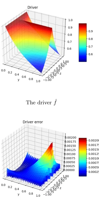
To construct our local polynomials approximation of ˆf, we use a linear spline interpolation in each direction, obtained by tensorization, and leading to a local approximation on the basis 1, y, z, yz on each mesh of a domain [0,1]×[−1,1]. Figure 1 displays the function ˆf and the error obtained by a discretization of 20×20 meshes.
The parameters affecting the convergence of the algorithm are:
• The couple of meshes (ny, nz) used in the spline representation of (23), where ny (resp. nz) is the number of linear spline meshes for they (resp.z) discretization.
• The number of time stepsNh.
• The grid and the interpolation used onXatt0= 0 and for all datesti,i= 1, . . . , Nh. Note that the size of the grid has to be adapted to the value ofT, because of the diffusive feature of (2). All interpolations are achieved with the StOpt library (see [9, 10]) using a modified quadratic interpolator as in [19]. In the following, ∆xdenotes the mesh of the space discretization.
• The time step is set to 0.002 and we use an Euler scheme to approximate (2).
• The accuracy of the estimation of the expectations appearing in our algorithm. We compute the empirical standard deviation θ associated to each Monte Carlo estimation of the expectation in (21).
We try to fix the number ˆM of samples such that θ/pMˆ does not exceed a certain level, fixed at 0.000125, at each point of our grid. We cap this number of simulations at 5105.
• The intensity, set to 0.4, of the exponential distribution used to define the random variables (δk)k∈K. Finally, we takeM = 1 in the definition ofR.
We only perform one Picard iteration with initial prior (˜u0,v˜0) = (g, Dgσ).
On the different figures below, we plot the errors obtained onXfor different values ofNh, (ny, nz) and ∆x. We first use 20 time steps and an interpolation step of 0.1 In figure 2, we display the error as a function of the number of spline meshes. We provide two plots:
• On the left-hand side,ny varies above 5 andnz varies above 10,
• On the right-hand side, we add (ny, nz) = (5,5). It leads to a maximal error of 0.11, showing that a quite good accuracy in the spline representation inz is necessary.
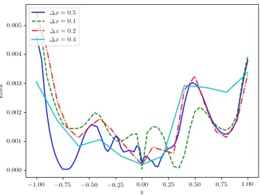
In figure 3, we plot the error obtained with (ny, nz) = (20,10) and a number of time steps equal toNh= 20, for different values of ∆x: the results are remarkably stable with the interpolation space discretization. In Figure 4, we finally let the number of time stepsNh vary. Once again we give two plots:
The driver ˆf
Error on the driver due to the linear spline representation.
Figure 1. The driver ˆf and its linear spline representation error for 20×20 splines.
• one with small values ofNh.
The results clearly show that the algorithm produces bad results when Nh is too small: the time steps are too large for the branching method. In this case, it exhibits a large variance. When Nh is too large, then interpolation errors propagate leading also to a deterioration of our estimations. Numerically, it can be checked that the face-lifting procedure is in most of the cases useless when only one Picard iteration is used:
• When the variance of the branching scheme is small, the face-lifting and truncation procedure has no effect,
• When the variance becomes too large, the face-lifting procedure is regularizing the solution and this permits to reduce the error due to our interpolations.
In figure 5, we provide the estimation with and without face-lifting, obtained withNh= 10, (ny, nz) = (20,10) and a space discretization ∆x= 0.1.
Figure 2. Error plot depending on the couple (ny, nz) for 20 time steps, a space discretization ∆x= 0.1.
Figure 3. Error plot depending on ∆xfor (ny, nz) = (20,10),Nh= 20.
3.2.
Extension to higher dimensions.
We extend the previous example to dimension 2 and 3. Forx∈Rd, We consider the SDE with coefficients:
µ(x) = (η(x1), . . . , η(xd)), withη(x) =−0.5(x+ 0.2),
andσ(x) is a diagonal matrix with fori= 1, . . . , d,
Figure 4. Error plot depending on Nhfor (ny, nz) = (20,10), a space discretization ∆x= 0.1
Figure 5. Error plot forNh= 10 for (ny, nz) = (20,10), a space discretization ∆x= 0.1 with and without face-lifting.
We keep a maturity ofT = 1 and the non linearity is given by:
f(t, x, y, z) = ˜f(y, z) +1 2e
t−T
2 cos(
d
X
i=1
xi) d
X
i=1
σ(xi)2
2 −
1
2(1 + cos( d
X
i=1
xi)) + sin( d
X
i=1
xi) d
X
i=1
η(xi)
!
− d
2 + 0.5|sin(Pd
i=1xi)(1 + cos(P d
i=1xi)))|et−T
,
where
˜
f(y, z) =1 2
d
X
i=1
ˆ
Notice that, due to the structure of ˜f, we can use the two-dimensional spline representation of the previous example for ˆf and thus avoid the use ofd+ 1-dimensional spline giving some more expensive methods.
The analytical solution corresponding tog(x) = 1+cos( Pd
i=1xi)
2 is given by
u(t, x) = 1 + cos(
Pd
i=1xi)
2 e
t−T
2 .
We take the following parameters :
• (ny, nz) = (20,10),
• ∆x= 0.2 and thed-dimensional modified quadratic interpolator of [19] is used for interpolation in grids, • 20 time steps.
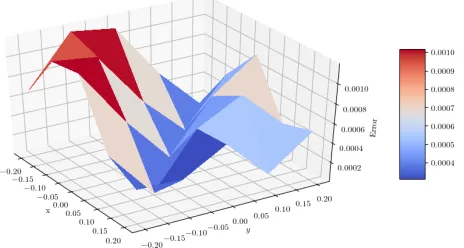
All the other parameters for the resolution are the same as in the previous section. On figure 6, we plot the error associated to the resolution of equation (2) for the two-dimensional case att= 0 on the grid for different
X0= (x, y). The solution is obtained in 60 seconds using a cluster of 224 cores. At last we calculate the solution
Figure 6. Error on the two dimensional case.
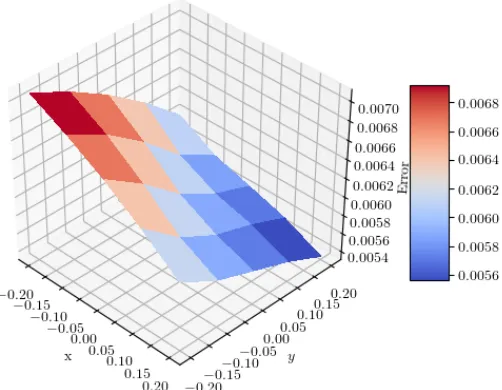
of the PDE in 3D. On a grid [−0.2,0,2]3, the maximum error associated to the resolution of equation (2) is 0.00747. Forz= 0 we plot the error obtained as a function of (x, y) on the figure 7. The solution is obtained in 900 seconds using a cluster of 224 cores.
A.
Appendix
A.1.
A priori estimates for the Picard iteration scheme
In this section, we let ∇X be the tangent process associated toX on [0, T] by
∇X0=Id, d∇Xt=Dµ(Xt)∇Xtdt+ d
X
i=1
Dσi(Xt)∇XtdWti,
and we define
Nst:=
Z s
t 1
s−t(σ(Xr) −1∇X
r)>dWr
>
Figure 7. Error on the three dimensional case forz= 0.
fort≤s≤T. Standard estimates lead to
Et[kNstk]≤Cµ,σ(s−t)−
1
2 fort≤s≤T, (25)
for some Cµ,σ>0 that only depends on kµk∞,kσk∞,kDµk∞,kDσk∞,a0 in (3) andT. In particular, it does
not depend onkX0k. Up to changing this constant, we may assume that
Et[k∇Xs∇Xt−1k]≤e
Cµ,σ(s−t) fort≤s≤T. (26)
Set
DMh◦ :=Rd× {(y, z)∈R×Rd:|y| ∨ kz>σ−1k ≤Mh◦} 2.
and letMh◦≥M andh◦∈(0, T] be such that
Mh◦≥M+ sup
DMh
◦
|f◦|h◦. (27)
and
Mh◦≥M e
Cµ,σh◦+C
µ,σ sup
DMh
◦
|f◦|(h◦)12 (28)
The existence of h◦ andMh◦follows from (4) and (5). Note that they do not depend onX0.
Proposition A.1. Let g˜ : Rd →
R be bounded by M and M-Lipschitz. Fix T0 ∈ [0, h◦]. Let ( ˜U ,V˜) :
[0, T0]×Rd →
solution on[0, T0] to
˜
Y·= ˜g(XT0) + Z T0
·
f◦(Xs,Y˜s,Z˜s,( ˜U ,V˜)(s, Xs))ds−
Z T0
·
˜
Zs>dWs. (29)
It satisfies
|Y˜| ∨ kZ˜>σ(X)−1k ≤Mh◦on [0, T
0]. (30)
Moreover, there exists a bounded continuous map(˜u,v˜) : [0, T0]×Rd→R×Rd such thatY˜ = ˜u(·, X)on [0, T0] P-a.s. and Z˜= ˜v(·, X)dt×dP-a.e. on[0, T0]×Ω. It satisfiesv˜>=Duσ˜ on[0, T0).
Proof. We construct the required solution by using Picard iterations. We set ( ˜Y0,Z˜0) = (y, Dy)(·, X), and
define recursively on [0, T0] the couple ( ˜Yn+1,Z˜n+1) as the unique solution of
˜
Y·n+1= ˜g(XT0) + Z T0
·
f◦(Xs,Y˜sn,Z˜ n
s,( ˜U ,V˜)(s, Xs))ds−
Z T0
·
( ˜Zsn+1)>dWs,
whenever it is well-defined. It is the case forn= 0. We now assume that ( ˜Yn,Z˜n) is well-defined and such that |Y˜n| ∨ kσ(X)−1Z˜nk ≤M
h◦ on [0, T
0] for some n≥0. Then,
|Y˜·n+1| ≤ kg˜k∞+ sup DMh◦
|f◦|h◦≤Mh◦,
in which we used (27) for the second inequality. On the other hand, up to using a mollifying argument, one can assume that ˜gisCb1and that (U, V) is Lipschitz. Then, it follows from the same arguments as in [15, Theorem 3.1, Theorem 4.2] that ˜Zn+1 admits the representation
( ˜Ztn+1)>=Et
D˜g(XT0)∇XT0∇Xt−1σ(Xt)
+Et
" Z T0
t
f◦(Xs,Y˜sn,Z˜ n
s,(U, V)(s, Xs))Nstds
# σ(Xt).
By combining the above together with (25) and (26), we obtain that
k( ˜Ztn+1)>σ(Xt)−1k ≤M eCµ,σ(T
0−t)
+Cµ,σ sup
DMh
◦
|f◦|(h◦) 1 2 ≤Mh
◦,
in which we used (28) for the second inequality. The above proves that the sequence ( ˜Yn,Z˜n)n≥0 is uniformly
bounded on [0, T0]. Therefore, we can consider f◦ as a Lipschitz generator, and hence ( ˜Yn,Z˜n)n≥0 is in fact a
Picard iteration that converges to a solution of (29) with the same bound.
The existence of the maps ˜uand ˜vsuch that ˜v> =Duσ˜ follows from [15, Theorem 3.1] applied to (29) when (˜g, f◦(·, y, z,(U, V)(t,·))) isCb1, uniformly in (t, y, z)∈[0, T]×Rd+1. The representation result of [15, Theorem 4.2] combined with a simple approximation argument, see e.g. [8, (ii) of the proof of Proposition 3.2], then shows
that the same holds on [0, T0) under our conditions.
A.2.
Proof of the representation formula
We adapt the proof of [13, Theorem 3.12] to our context. We proceed by induction. In all this section, we fix
and assume that the result of Proposition 2.1 holds up to rankm−1≥0 on [0, T] (with the conventionU0
· =y, V0
· :=Dy), and up to rankmon [ti+1, T]. In particular, we assume that ˜um(ti+1,·) = ¯um(ti+1,·).
We fix%= 4 and define
C1,%:=M%∨ sup
t≤s, x∈Rd, q=1,···,q◦,kξk≤M
E h
ξ·(X
t,x s −x)
bq(x)· Wt,x,s
%i ,
C2,%:= sup
t≤s≤ti+1, x∈Rd, q=1,···,q◦
E h
√
s−t bq(x)· Wt,x,s
%i
where
Wt,x,s:= 1
s−t Z s
t
σ−1(Xrt,x)∇Xrt,x> dWr
in which∇Xt,x is the tangent process ofXt,xwith initial conditionI
d att. We then set
ˆ
C1,%:=
C1,% ¯
F(T)%−1, Cˆ2,%:=C2,%j◦ sup
j≤j◦,`∈L,t∈(0,h◦]
kcj,`k∞ p`
t−%/(2(%−1))
ρ(t)
%−1 .
Since ¯F is non-increasing and ˜um(t
i+1,·) = ¯um(ti+1,·) is bounded byM andM-Lipschitz, direct computations
imply that
E[|Ut,xm| %]∨
EkVt,xmk %]≤
E h Y
k∈Kt ˆ
C1,% ¯
F(t−Tk−)
Y
k∈K¯t\Kt
ˆ
C2,%
pξkρ(δk)
i
. (31)
We first estimate the right-hand side, see (34) below.
Let us denote byCbdgthe constant in the Burkholder-Davis-Gundy inequality such thatEsup0≤t≤T|Mt|%]≤
CbdgE[(hMiT)
%
2] for any continuous martingaleM withM0= 0. Denote further
C0:= (3×3)%−1 1 + (%/(%−1))% 1 + (1 +|λ¯DµT|%eCQT),
where ¯λDµ the largest eigenvalue of the matrix Dµ, ¯λDσ the largest eigenvalue of the matrix Dσi, i≤d, and
CQ:=%¯λDµ+d%(%−1)¯λDσ/2. Define also ¯λ(σσ>)−1 as the largest eigenvalue of matrix (σσ>)−1. Lemma A.2. Under the Assumptions of Proposition 2.1,
ˆ
C1,%≤Cˆ1:= 2
1∨M∨2%−1(M
√
d)%C0+kµk%T
%
2CBDGC0 ¯λ
(σσ>)−1 %2,
and
ˆ
C2,%≤Cˆ2:=Cbdg C0 λ¯(σσ>)−1
%
2.
Proof. Let ˜b∈Rd be a fixed vector. Set Qt,x:=∇Xt,x˜b. Then, it follows from direct computations that
E h
max
[t,ti+1]
kQt,xk%i≤C
0k˜bk%.
Further, remember that each bq is assumed to be bounded by 1, so thatkbqσ−1k2 is uniformly bounded by ¯
λ(σσ>)−1. Then, direct computations lead to
C1,%≤1∨M%∨2%−1
C0+kµkqT
%
2CbdgC0 λ¯(σσ>)−1
%
2,
and
C2,%≤Cbdg C0 λ¯(σσ>)−1
%
It remains to use our specific choice ofρand (p`)`∈L in Proposition 2.1 to conclude. Let us now chooseh0◦ andMh0
◦ such that
h0◦ < 1∧ Cˆ
−(|L|−1) 1
(|L|+ 1)(|L| −1) ˆC2
, (32)
and
(Mh0 ◦)
4 := Cˆ1−|L|
1 −h
0
◦(|L|+ 1)(|L| −1) ˆC2
(1−|L|)−1
. (33)
Lemma A.3. Let the conditions of Proposition 2.1 hold. Then, the ordinary differential equation η0(t) =
P
`∈LCˆ2η(t)
k`k1 with initial condition η(0) = ˆC
1 ≥ 1 has a unique solution on [0, h0◦], and it is bounded by
(Mh0 ◦)
2. Moreover,
E h Y
k∈Kt ˆ
C1
¯
F(t−Tk−)
Y
k∈K¯t\Kt
ˆ
C2
pξkρ(δk)
i
≤ η(t) ≤ (Mh0 ◦)
4, (34)
for allt∈[0, h0◦].
Proof. The result follows from exactly the same arguments as in [3, Lemma A.1].
We can now conclude the proof of Proposition 2.1.
Proof of Proposition 2.1. In view of (31), Lemma A.3 implies that{|Um
t,x|2+kVt,xmk2,(t, x)∈[ti, ti+1)×Rd}
is uniformly integrable (with a bound that does not depend oni < Nhfor 0< h≤h0◦ ). Then, arguing exactly
as in [3, Proposition A.2] leads to ˜um = ¯um on [ti, ti+1). Combined with [13, Proposition 3.7], the uniform
integrability also implies that Du˜m = ˜vmσ on (ti, ti+1)×Rd, and one can conclude from Theorem 1.3 that
˜
vm= ˜um on (t
i, ti+1)×Rd. By the induction hypothesis of the beginning of this section, this proves that the
statements of Proposition 2.1 hold.
Remark A.4. The constants ˆC1and ˆC2 (and henceh0◦ andMh0
◦) are clearly not optimal for applications. For
instance, if σ≡σ◦, for some non-degenerate constant matrix, the constants C1,% andC2,% can be significantly simplified as shown in [13, Remark 3.9].
This work has benefited from the financial support of the Initiative de Recherche “M´ethodes non-lin´eaires pour la gestion des risques financiers” sponsored by AXA Research Fund.
Bruno Bouchard and Xavier Warin acknowledge the financial support of ANR project CAESARS (ANR-15-CE05-0024).
Xiaolu Tan acknowledges the financial support of the ERC 321111 Rofirm, the ANR Isotace (ANR-12-MONU-0013), and the Chairs Financial Risks (Risk Foundation, sponsored by Soci´et´e G´en´erale) and Finance and Sustainable Devel-opment (IEF sponsored by EDF and CA).
References
[1] V. Bally and P. Pages, Error analysis of the quantization algorithm for obstacle problems, Stochastic Processes & Their Applications, 106(1), 1-40, 2003.
[2] B. Bouchard, J.F. Chassagneux. Fundamentals and advanced techniques in derivatives hedging. Springer Universitext, 2016. [3] B. Bouchard, X. Tan , X. Warin and Y. Zou,Numerical approximation of BSDEs using local polynomial drivers and branching
processes, Monte Carlo Methods and Applications, to appear.
[4] B. Bouchard and N. Touzi,Discrete-time approximation and Monte-Carlo simulation of backward stochastic differential equa-tions, Stochastic Process. Appl., 111(2), 175-206, 2004.
[6] J.F. Chassagneux, R. Elie and I. Kharroubi, A numerical probabilistic scheme for super-replication with Delta constraints, arXiv, forthcoming.
[7] N. El Karoui, S. Peng, M.C. Quenez,Backward stochastic differential equations in finance, Mathematical finance 7(1), 1-71, 1997.
[8] E. Fourni´e, J.M. Lasry, , J. Lebuchoux, P.L. Lions, N. Touzi,Applications of Malliavin calculus to Monte Carlo methods in finance. Finance and Stochastics, 3(4), 391–412, 1999.
[9] H. Gevret, J. Lelong, X. Warin,The StOpt library,https://gitlab.com/stochastic-control/StOpt
[10] H. Gevret, J. Lelong, X. Warin ,STochastic OPTimization library in C++, EDF Lab, 2016.
[11] E. Gobet, J.P. Lemor, X. Warin,A regression-based Monte Carlo method to solve backward stochastic differential equations. The Annals of Applied Probability, 15(3), 2172-202, 2005.
[12] P. Henry-Labord`ere,Cutting CVA’s Complexity, Risk, 25(7), 67, 2012.
[13] P. Henry-Labordere, N. Oudjane, X. Tan, N. Touzi, X. Warin,Branching diffusion representation of semilinear PDEs and Monte Carlo approximation. arXiv preprint, 2016.
[14] P. Henry-Labordere, X. Tan, N. Touzi,A numerical algorithm for a class of BSDEs via the branching process. Stochastic Processes and their Applications, 28, 124(2), 1112-1140, 2014.
[15] J. Ma and J. Zhang,Representation theorems for backward stochastic differential equations. The annals of applied probability, 12(4), 1390–1418, 2002.
[16] H.P. McKean,Application of Brownian motion to the equation of Kolmogorov-Petrovskii-Piskunov, Comm. Pure Appl. Math., 28, 323-331, 1975.
[17] A.V. SkorokhodBranching diffusion processes, Theory of Probability & Its Applications, 9(3), 445-449, 1964.
[18] S. Watanabe,On the branching process for Brownian particles with an absorbing boundary, J. Math. Kyoto Univ. 4(2), 385-398, 1964.
[19] X. Warin, Some Non-monotone Schemes for Time Dependent Hamilton-Jacobi-Bellman Equations in Stochastic Control, Journal of Scientific Computing, 66(3), 1122-1147, 2016.
[20] X. Warin,Variations on branching methods for non linear PDEs, arXiv preprint arXiv:1701.07660, 2017